Introduction

In the field of bioinformatics and genomics, understanding the variations in gene expression across different experimental conditions is crucial for interpreting biological processes. The limma package is widely recognized for its powerful capabilities in fitting linear models to gene expression data, allowing researchers to evaluate differences due to experimental conditions.

However, many experimental designs involve repeated measurements from the same subjects, whether they are animals, human samples, or cells. These repeated measures introduce random effects, which must be accounted for to avoid biased results. Random effects occur when some variability in the data is due to differences between subjects or samples that are not directly related to the experimental conditions being studied.

This tutorial provides a step-by-step guide on how to build linear mixed models (LMM) using the limma package to incorporate random effects. You will learn how to adjust for these random variations, ensuring more accurate and reliable conclusions about gene expression.

What is effect of repeated measures?

Repeated measures refer to data collected from the same subjects at multiple time points or under different conditions. These designs result in correlated observations, as repeated measures on the same individual tend to share subject-specific traits. Ignoring this correlation can lead to incorrect conclusions since traditional methods assume independence between observations.

The use of repeated measures often reduces variability, as each subject serves as their own control, which increases the sensitivity of the analysis. This can lead to greater statistical power, enabling researchers to detect effects with fewer subjects. To handle the correlation between repeated observations, specialized methods such as Repeated Measures ANOVA, Linear Mixed Models (LMM), or Generalized Estimating Equations (GEE) are typically used.

What can linear mixed-effect model do?

A Linear Mixed-Effects Model (LMM) is used to analyze repeated measures data by accounting for both overall effects (like treatments or time) and individual differences between subjects. It helps manage the fact that repeated observations from the same person are related, and it can handle missing data or different time points for each person. This makes it a flexible tool for analyzing complex data.

In the context of gene expression analysis, LMMs can be used to model the effects of experimental conditions (e.g., treatment groups) while accounting for individual variability and correlations between repeated measurements. By incorporating random effects, LMMs provide a more accurate representation of the underlying data structure, leading to more reliable results and improved statistical power.

Prerequisites

Before proceeding with this tutorial, you should have a basic understanding of linear models, gene expression analysis, and the R programming language. Familiarity with the limma package and its functions is recommended but not required.

To follow along with the code examples, you will need to have R and RStudio installed on your computer. You can download R from the Comprehensive R Archive Network (CRAN) and RStudio from the RStudio website. Additionally, you will need to install the limma package, which can be done using the BiocManager package.

The R package limma is used for linear models and differential expression analysis. If you haven’t installed the package yet, you can do so by running the following code:

    # Install the biocManager package 
    # install.packages("BiocManager") 
    # Install the limma package 
    # BiocManager::install("limma", force = TRUE)  

    library(limma) # For linear models and differential expression analysis 
    library(ggplot2) # For data visualization 
    library(gridExtra)

Code Structure

This tutorial is divided into four main steps:

Simulate Example Data: We will generate example data with repeated measures to demonstrate the use of linear mixed-effect models with the limma package.
Fit Linear Models with limma: We will fit linear models to the example data using the limma package, considering different model configurations.
Evaluate the Block Effect: We will extract differentially expressed genes and visualize the coefficients and confidence intervals for the fixed effects of treatment on gene expression.
Evaluate Model Robustness: We will evaluate the assumptions of homoscedasticity and linearity by examining the residuals and checking the normality of residuals using Q-Q plots.

Step 1 - Simulate example data

In this step, we will simulate example data to demonstrate the use of linear mixed-effect models with the limma package.

The example data will consist of gene expression data for 10 individuals per group (control and treatment groups), with 2 samples (repeative measures) per individual.

We will simulate the following variables for each sample: 1. people: A numeric variable representing the individual ID 2. treatment: A factor variable indicating the treatment group (0 = Control, 1 = Treatment) 3. gender: A factor variable representing

We will also simulate gene expression data for 5 genes, from normal distributions with different means and standard deviations for the control and treatment groups.

The gene expression data will be combined into a single data frame, with the genes as rows and the samples as columns.

    # Simulate example data
    set.seed(123)

    # Define variables
    people <- rep(c(1:10), each = 2) # 10 people, 2 samples per person 
    treatment <- factor(rep(c(0, 1), each = 10))  # 0 = Control, 1 = Treatment
    gender <- factor(sample(c("Male", "Female"), 20, replace = TRUE))  # Gender
    genes <- paste0("Gene", 1:5)

    # Simulate gene expression matrix for treatment group
    gene_expression_treatment <- matrix(rnorm(50, mean = 10, sd = 2), nrow = 5, dimnames = list(genes, 1:10)) 
    print(gene_expression_treatment)

    ##               1         2        3         4         5         6         7         8         9        10
    ## Gene1 12.448164 13.573826 7.864353  6.626613 10.852928 11.377281  8.610586  7.753783 10.506637 13.032941
    ## Gene2 10.719628 10.995701 9.564050 11.675574  9.409857 11.107835  9.584165  9.194230  9.942906  6.902494
    ## Gene3 10.801543  6.066766 7.947991 10.306746 11.790251  9.876177  7.469207  9.066689  9.914259 11.169227
    ## Gene4 10.221365 11.402712 8.542218  7.723726 11.756267  9.388075 14.337912 11.559930 12.737205 10.247708
    ## Gene5  8.888318  9.054417 8.749921 12.507630 11.643162  9.239058 12.415924  9.833262  9.548458 10.431883

    # Simulate gene expression matrix for control group 
    gene_expression_control <- matrix(rnorm(50, mean = 5, sd = 2), nrow = 5, dimnames = list(genes, 1:10)) 
    print(gene_expression_control)

    ##              1        2         3        4        5        6        7        8        9       10
    ## Gene1 5.759279 5.607057 4.0179377 7.051143 5.011528 5.663564 6.987008 3.799481 3.579187 4.909945
    ## Gene2 3.995353 5.896420 0.3816622 4.430454 5.770561 7.193678 6.096794 9.374666 5.513767 3.430191
    ## Gene3 4.333585 5.106008 7.0114770 2.558565 4.258680 5.870363 5.477463 8.065221 4.506616 1.664116
    ## Gene4 2.962849 6.844535 3.5815985 5.362607 6.288753 4.348137 3.744188 4.528599 4.304915 4.239547
    ## Gene5 2.856418 9.100169 3.6239828 4.722217 4.559027 7.297615 7.721305 2.947158 3.096763 6.837993

    # Combine the gene expression data 
    gene_expression <- cbind(gene_expression_treatment, gene_expression_control)

    # Create a data frame with the gene expression data 
    expression_data <- data.frame(gene_expression, row.names = genes)
    colnames(expression_data) <- paste0("sample", 1:20) 

    # Print the expression data
    print(expression_data) 

    ##         sample1   sample2  sample3   sample4   sample5   sample6   sample7   sample8   sample9  sample10 sample11 sample12  sample13 sample14 sample15 sample16 sample17
    ## Gene1 12.448164 13.573826 7.864353  6.626613 10.852928 11.377281  8.610586  7.753783 10.506637 13.032941 5.759279 5.607057 4.0179377 7.051143 5.011528 5.663564 6.987008
    ## Gene2 10.719628 10.995701 9.564050 11.675574  9.409857 11.107835  9.584165  9.194230  9.942906  6.902494 3.995353 5.896420 0.3816622 4.430454 5.770561 7.193678 6.096794
    ## Gene3 10.801543  6.066766 7.947991 10.306746 11.790251  9.876177  7.469207  9.066689  9.914259 11.169227 4.333585 5.106008 7.0114770 2.558565 4.258680 5.870363 5.477463
    ## Gene4 10.221365 11.402712 8.542218  7.723726 11.756267  9.388075 14.337912 11.559930 12.737205 10.247708 2.962849 6.844535 3.5815985 5.362607 6.288753 4.348137 3.744188
    ## Gene5  8.888318  9.054417 8.749921 12.507630 11.643162  9.239058 12.415924  9.833262  9.548458 10.431883 2.856418 9.100169 3.6239828 4.722217 4.559027 7.297615 7.721305
    ##       sample18 sample19 sample20
    ## Gene1 3.799481 3.579187 4.909945
    ## Gene2 9.374666 5.513767 3.430191
    ## Gene3 8.065221 4.506616 1.664116
    ## Gene4 4.528599 4.304915 4.239547
    ## Gene5 2.947158 3.096763 6.837993

Step 2 - Fit linear models with limma

In this step, we will fit linear models to the example data using the limma package. We will consider three different models:

Model 1: Treatment as the only predictor variable
Model 2: Treatment and gender as covariates
Model 3: Treatment and gender as covariates with repeated measures

In limma, block effects can be used to account for non-independent samples, such as technical replicates or paired samples. You can use the duplicateCorrelation() function to model the correlation between samples within the same block.

    #------Model 1: Treatment as the only predictor variable------# 
    # Create model matrix (with treatment as the only predictor variable)  
    design_1 <- model.matrix(~ treatment, data = expression_data) 
    # Fit the linear model
    fit_1 <- lmFit(expression_data, design_1)  
    # Apply empirical Bayes moderation
    fit_1_ebayes <- eBayes(fit_1)


    #------Model 2: Treatment and Gender as covariates------# 
    # Create design matrix (treatment and gender as covariates)
    design_2 <- model.matrix(~ treatment + gender, data = expression_data)
    # Fit the linear model for each gene
    fit_2 <- lmFit(expression_data, design_2)
    # Apply empirical Bayes moderation
    fit_2_ebayes <- eBayes(fit_2)


    #------Model 3: Treatment and Gender as covariates with repeated measures------# 
    # Model the correlation between samples within the same block (repeated measures) 
    corfit <- limma::duplicateCorrelation(gene_expression, design_2, block = people) 
    # Incorprate the block effect in the model 
    fit_3 <- lmFit(gene_expression, design_2, block = people, correlation = corfit$consensus)
    # Apply empirical Bayes moderation
    fit_3_ebayes <- eBayes(fit_3) 

The corfit$consensus object contains the correlation structure of the repeated measures, which is used in the lmFit function to account for the correlation between samples from the same individual. It is an estimate of the average intra-block correlation. If the value is close to zero, the block effect is weak or negligible. A higher value (closer to 1) indicates a stronger correlation within blocks, meaning the block effect is significant.

In this case, the block effect is not significant, as the correlation is close to zero (approximately, 0.01).

Step 3 - Evaluate the Block Effect

Extract top differentially expressed genes

In this step, we will extract the top differentially expressed genes from the fitted models. We will use the topTable function to extract the results, including the log fold change, moderated t-statistic, raw p-value, adjusted p-value (FDR), and log-odds that the gene is differentially expressed.

    # Extract top differentially expressed genes
    topTable(fit_1_ebayes, number = Inf, adjust.method = "BH", sort.by = "P") 

    ## Removing intercept from test coefficients

    ##           logFC  AveExpr         t      P.Value    adj.P.Val         B
    ## Gene4 -6.171139 7.706142 -7.430413 5.986052e-11 2.993026e-10 20.276398
    ## Gene1 -5.026098 7.751662 -6.051717 3.234941e-08 7.859775e-08 11.366624
    ## Gene5 -4.954939 7.753734 -5.966037 4.715865e-08 7.859775e-08 10.873058
    ## Gene2 -4.701290 7.558999 -5.660628 1.776199e-07 2.220249e-07  9.170996
    ## Gene3 -4.555676 7.163048 -5.485301 3.752867e-07 3.752867e-07  8.234286

    # Show results
    topTable(fit_2_ebayes)

    ## Removing intercept from test coefficients

    ##       treatment1  genderMale  AveExpr        F      P.Value    adj.P.Val
    ## Gene4  -6.174442 -0.03303168 7.706142 27.05854 1.772654e-12 8.863272e-12
    ## Gene1  -4.913836  1.12261968 7.751662 18.82582 6.668838e-09 1.667210e-08
    ## Gene5  -5.047809 -0.92870157 7.753734 18.04422 1.457123e-08 2.428538e-08
    ## Gene2  -4.660927  0.40362347 7.558999 15.81690 1.351472e-07 1.689340e-07
    ## Gene3  -4.570297 -0.14621287 7.163048 14.76065 3.886259e-07 3.886259e-07

    # Show results
    topTable(fit_3_ebayes) 

    ## Removing intercept from test coefficients

    ##       treatment1  genderMale  AveExpr        F      P.Value    adj.P.Val
    ## Gene4  -6.173634 -0.02495011 7.706142 26.77375 2.356711e-12 1.178356e-11
    ## Gene1  -4.914731  1.11367369 7.751662 18.62289 8.169239e-09 2.042310e-08
    ## Gene5  -5.047331 -0.92392051 7.753734 17.85445 1.761614e-08 2.936023e-08
    ## Gene2  -4.660333  0.40956206 7.558999 15.65513 1.588780e-07 1.985975e-07
    ## Gene3  -4.570291 -0.14614599 7.163048 14.60561 4.538018e-07 4.538018e-07

Parameters Interpretation: - logFC: Log fold change of the gene expression between conditions. - AveExpr: Average expression of the gene across all samples. - t: Moderated t-statistic. - P.Value: Raw p-value. - adj.P.Val: Adjusted p-value (FDR). - B: Log-odds that the gene is differentially expressed.

If including the block effect changes the results substantially (e.g., differentially expressed genes, p-values), then the block effect is important in your model. Otherwise, if there is minimal change, the block effect may not significantly impact the model.

In this case, the block effect does not significantly affect the results, as the top differentially expressed genes are similar across the models. In contrast, the covariate, gender has a significant impact on the results, as the top differentially expressed genes differ between Model 1 and Model 2.

Visualize the coefficients and CI

In this step, we will visualize the coefficients and confidence intervals for the fixed effects of treatment on gene expression. We will compare the results from Model 1, Model 2, and Model 3.

    # Define a function to extract the coefficients and confidence intervals 
    extract_coef_ci <- function(fit) {
      coef_df <- data.frame(
        Gene = rownames(fit$coefficients),
        Estimate = fit$coefficients[, "treatment1"],
        CI_Lower = fit$coefficients[, "treatment1"] - 1.96 * fit$stdev.unscaled[, "treatment1"] * fit$sigma,
        CI_Upper = fit$coefficients[, "treatment1"] + 1.96 * fit$stdev.unscaled[, "treatment1"] * fit$sigma
      )
      return(coef_df)
    }

    # Extract coefficients and confidence intervals for Model 1 - 3 
    coef_df_1 <- extract_coef_ci(fit_1_ebayes)
    coef_df_2 <- extract_coef_ci(fit_2_ebayes)
    coef_df_3 <- extract_coef_ci(fit_3_ebayes)

    # Prepare the data for plotting 
    coef_df_1$model <- "Model_1"
    coef_df_2$model <- "Model_2" 
    coef_df_3$model <- "Model_3" 

    coef_df <- rbind(coef_df_1, coef_df_2, coef_df_3) 
    print(coef_df)  

    ##         Gene  Estimate  CI_Lower  CI_Upper   model
    ## Gene1  Gene1 -5.026098 -6.710451 -3.341746 Model_1
    ## Gene2  Gene2 -4.701290 -6.404071 -2.998508 Model_1
    ## Gene3  Gene3 -4.555676 -6.179768 -2.931585 Model_1
    ## Gene4  Gene4 -6.171139 -7.610268 -4.732010 Model_1
    ## Gene5  Gene5 -4.954939 -6.629405 -3.280472 Model_1
    ## Gene11 Gene1 -4.913836 -6.572943 -3.254729 Model_2
    ## Gene21 Gene2 -4.660927 -6.411613 -2.910241 Model_2
    ## Gene31 Gene3 -4.570297 -6.248554 -2.892041 Model_2
    ## Gene41 Gene4 -6.174442 -7.662748 -4.686136 Model_2
    ## Gene51 Gene5 -5.047809 -6.722954 -3.372663 Model_2
    ## Gene12 Gene1 -4.914731 -6.578634 -3.250828 Model_3
    ## Gene22 Gene2 -4.660333 -6.417573 -2.903094 Model_3
    ## Gene32 Gene3 -4.570291 -6.258486 -2.882096 Model_3
    ## Gene42 Gene4 -6.173634 -7.668705 -4.678563 Model_3
    ## Gene52 Gene5 -5.047331 -6.737661 -3.357000 Model_3

    # Plot the fixed effects with confidence intervals, comparing Model 1 - 3 
    pd <- position_dodge(width = 0.2) # Position dodge for better visualization 

    ggplot(coef_df, aes(x = Gene, y = Estimate, color = model)) +
      geom_point(position = pd, size = 3) +
      geom_errorbar(aes(ymin = CI_Lower, ymax = CI_Upper), width = 0.2, position = pd) + # Error bars for confidence intervals 
      labs(title = "Fixed Effects of Treatment on Gene Expression",
           x = "Gene",
           y = "Estimate (Treatment Effect)") +
      theme_minimal() +
      theme(legend.position = "top") 

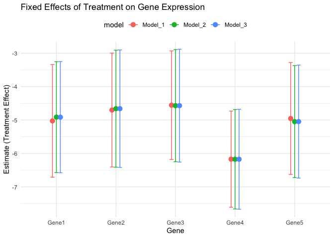
The plot shows the fixed effects of treatment on gene expression, with confidence intervals for Model 1 - 3. The coefficients represent the estimated treatment effect on gene expression, and the confidence intervals indicate the uncertainty around the estimates.

The gene expression of Genes 1 - 5 are significantly downregulated in the treatment group compared to the control group, as the confidence interval does not include zero. The confidence intervals provide a range of plausible values for the treatment effect, taking into account the uncertainty in the estimates.

Step 4 - Evaluate model robustness

This step evaluates the assumptions of homoscedasticity and linearity by examining the residuals. If the residuals are randomly distributed around zero and show no clear patterns, the assumptions are met. If there are patterns or trends in the residuals, further investigation may be needed to address model assumptions.

    # Plot the residuals

    # Create a functiont to plot fitted values vs residuals 
    plot_residuals <- function(fit, data) {
      residuals_df <- data.frame(
        Residuals = as.vector(residuals(fit, y = data)), 
        Fitted = as.vector(fitted(fit))
      ) 
      
      ggplot(residuals_df, aes(x = Fitted, y = Residuals)) +
        geom_point() +
        geom_hline(yintercept = 0, linetype = "dashed") +
        labs(title = "Residuals vs Fitted Values",
             x = "Fitted Values",
             y = "Residuals") +
        theme_minimal()
    }

    # Combine the residual plots for Model 1 - 3
    grid.arrange(plot_residuals(fit_1, expression_data), 
                 plot_residuals(fit_2, expression_data), 
                 plot_residuals(fit_3, gene_expression), 
                 nrow = 3) 

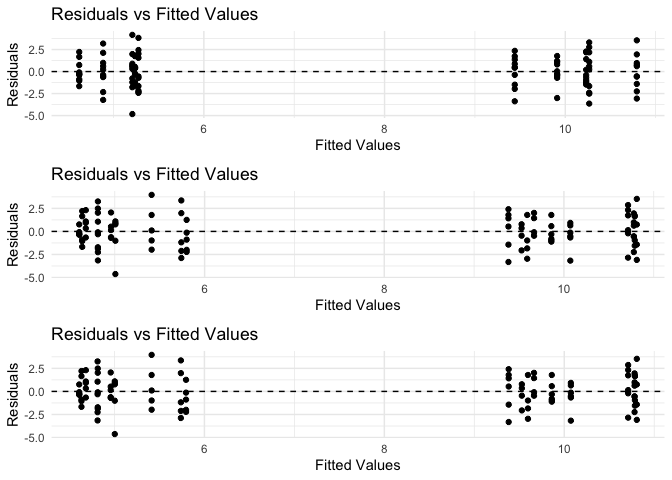
In this case, the residual plots show no clear patterns or trends, indicating that the assumptions of homoscedasticity and linearity are met for Model 1 - 3.

    # Check the normality of residuals using Q-Q plots 
    par(mfrow = c(3, 1)) 
    qqnorm(residuals(fit_1, y = expression_data)) 
    qqline(residuals(fit_1, y = expression_data)) 

    qqnorm(residuals(fit_2, y = expression_data)) 
    qqline(residuals(fit_2, y = expression_data))

    qqnorm(residuals(fit_3, y = gene_expression)) 
    qqline(residuals(fit_3, y = gene_expression)) 

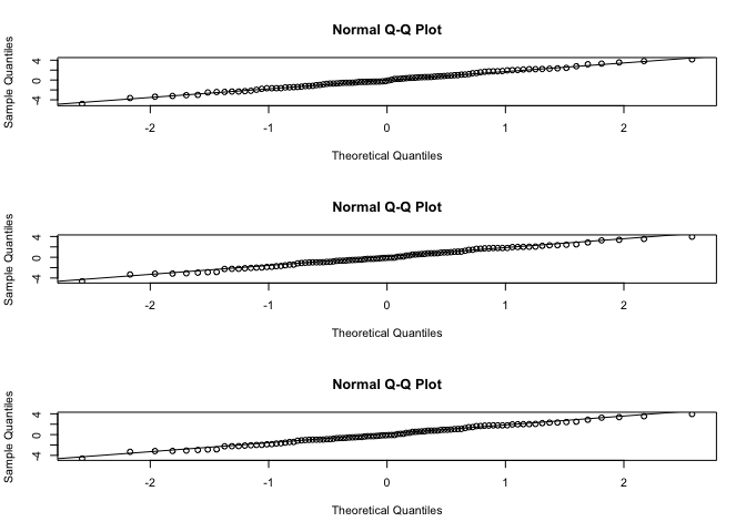
The residuals are randomly distributed around zero, with no systematic deviations from the assumptions.

Conclusion

In this tutorial, we demonstrated how to fit linear mixed-effect models with the limma package in R. We simulated example data with repeated measures and applied linear models with different covariates and block effects. We evaluated the block effect, extracted differentially expressed genes, visualized the coefficients, and assessed model robustness.

Linear mixed-effect models are useful for analyzing data with repeated measures or nested structures, where samples are not independent. By incorporating random effects and block effects, we can account for the correlation between samples and improve the accuracy of the statistical analysis.

This tutorial is for demonstration purpose, although the block efffect is not significant. You can apply similar steps to analyze your own data with linear mixed-effect models using the limma package in R.

Sessoin Info

    sessionInfo()

    ## R version 4.3.3 (2024-02-29)
    ## Platform: aarch64-apple-darwin20 (64-bit)
    ## Running under: macOS 15.0
    ## 
    ## Matrix products: default
    ## BLAS:   /System/Library/Frameworks/Accelerate.framework/Versions/A/Frameworks/vecLib.framework/Versions/A/libBLAS.dylib 
    ## LAPACK: /Library/Frameworks/R.framework/Versions/4.3-arm64/Resources/lib/libRlapack.dylib;  LAPACK version 3.11.0
    ## 
    ## locale:
    ## [1] en_US.UTF-8/en_US.UTF-8/en_US.UTF-8/C/en_US.UTF-8/en_US.UTF-8
    ## 
    ## time zone: America/Edmonton
    ## tzcode source: internal
    ## 
    ## attached base packages:
    ## [1] stats     graphics  grDevices utils     datasets  methods   base     
    ## 
    ## other attached packages:
    ## [1] rmarkdown_2.26 gridExtra_2.3  limma_3.58.1   shiny_1.9.1    ggplot2_3.5.0  bookdown_0.41 
    ## 
    ## loaded via a namespace (and not attached):
    ##  [1] sass_0.4.9          utf8_1.2.4          generics_0.1.3      digest_0.6.35       magrittr_2.0.3      evaluate_0.23       grid_4.3.3          fastmap_1.2.0      
    ##  [9] jsonlite_1.8.8      promises_1.2.1      BiocManager_1.30.25 fansi_1.0.6         scales_1.3.0        jquerylib_0.1.4     cli_3.6.2           rlang_1.1.3        
    ## [17] munsell_0.5.0       withr_3.0.0         cachem_1.1.0        yaml_2.3.8          tools_4.3.3         memoise_2.0.1       dplyr_1.1.4         colorspace_2.1-1   
    ## [25] httpuv_1.6.15       vctrs_0.6.5         R6_2.5.1            mime_0.12           lifecycle_1.0.4     pkgconfig_2.0.3     pillar_1.9.0        bslib_0.6.2        
    ## [33] later_1.3.2         gtable_0.3.4        glue_1.7.0          Rcpp_1.0.12         statmod_1.5.0       xfun_0.48           tibble_3.2.1        tidyselect_1.2.1   
    ## [41] highr_0.10          rstudioapi_0.16.0   knitr_1.45          farver_2.1.1        xtable_1.8-4        htmltools_0.5.8     labeling_0.4.3      compiler_4.3.3