Modeling Diagnostic Delays in Rare Disease: A Survival Analysis Case Study in Python
Introduction: Why Survival Analysis?
Rare diseases often come with a hidden burden—the delay in diagnosis. For patients with acid sphingomyelinase deficiency (ASMD), a genetic disorder with highly variable onset and progression, the diagnostic journey can be long and uncertain. Those with chronic neurovisceral ASMD (NPD A/B) and chronic visceral ASMD (NPD B) may face years before receiving a definitive diagnosis, impacting their treatment options and long-term health outcomes.
But how long do these delays typically last? Can we quantify the diagnostic journey and predict the likelihood of diagnosis at different time points?
This is where survival analysis comes in. By modeling time-to-diagnosis, we can estimate median diagnostic timelines, compare different patient subgroups, and even predict when a patient is most likely to receive a diagnosis based on their clinical history. In this article, I’ll walk through the fundamentals of survival analysis and share how I applied it to ASMD patient data using Python.
You can explore the full notebook and dataset to try the analysis yourself 🚀
My Learning Journey in Survival Analysis
Why I started exploring survival analysis
I became interested in survival analysis because it answers a critical question: How likely is an event (such as diagnosis) to occur at a given time point, considering different covariates?
This type of analysis is widely used in: • Disease progression modeling – Understanding how long it takes for a condition to worsen. • Precision medicine – Predicting patient outcomes based on medical history. • Clinical trials – Estimating time-to-recovery, disease recurrence, or survival rates.
Unlike conventional regression models, survival analysis can handle censored data—cases where the event of interest hasn’t occurred yet by the time of data collection. This makes it a powerful tool in both medical research and epidemiology.
Key takeaways from my learning process
As I explored survival analysis, I focused on three major areas:
- Understanding the statistical foundations
- The concept of censored data and why it’s important.
- Common survival models: Kaplan-Meier curves, parametric regression models, and Cox proportional hazards models.
- Model selection using AIC to determine the best fit.
- Implementing survival analysis in Python
- Learning by reproducing examples from tutorials and documentation.
- Using the lifelines library for survival modeling and visualization.
- Writing clean, reusable code for different types of survival models.
- Applying knowledge to a real-world case study
- Choosing the right statistical models: non-parametric, semi-parametric, or parametric.
- Interpreting model coefficients in the context of a medical study.
- Creating effective and insightful plots to communicate results.
How this method applies beyond ASMD
While this case study focuses on time-to-diagnosis in ASMD, the approach can be generalized to many other scenarios:
- The analysis workflow can be applied to different time-to-event studies.
- The parametric models used in survival analysis can be adjusted for other medical research questions.
- The Python code can be repurposed for different datasets with minimal modifications.
What this post covers
In this blog post, I’ll share:
✅ A beginner-friendly introduction to survival analysis.
✅ Helpful resources for learning survival analysis and Python implementation.
✅ A step-by-step case study using ASMD diagnosis data.
🚀 For the full code and interactive analysis, check out my Jupyter Notebook
Let’s dive in!
Fundamentals of Survival Analysis
What is survival analysis?
Survival analysis is a statistical approach used to model time-to-event data—where the outcome of interest is the time until an event occurs. This event could be time to disease relapse, time until a diagnosis, or even time to treatment failure. Despite the name, survival analysis isn’t just about survival—it’s about understanding when an event is likely to happen.
One of the key advantages of survival analysis is its ability to handle censored data—cases where:
- Left censoring occurs when the event happened before the study began, but the exact time is unknown.
- Right censoring happens when the event has not yet occurred by the end of the study period.
Traditional regression models struggle with these challenges, but survival models are specifically designed to account for incomplete data, making them essential in epidemiology, clinical research, and beyond.
Key concepts explained simply
Censoring: Not every subject in a study experiences the event of interest. Censoring allows us to include incomplete observations, making survival analysis more robust than conventional regression methods.
Kaplan-Meier Curve: A Kaplan-Meier curve provides a visual representation of survival probabilities over time. It plots:
- Time (X-axis) vs. Probability of event-free survival (Y-axis).
- It helps estimate how likely the event (e.g., diagnosis) will occur by a given time.
Log-Rank Test: A statistical test used to compare survival distributions between two or more independent groups. For example, it helps determine whether patients with different ASMD subtypes experience significantly different diagnostic delays.
Cox Proportional Hazards Model: A regression model that evaluates the effect of multiple variables on survival time. It helps answer questions like:
- Do certain clinical factors increase or decrease the likelihood of earlier diagnosis?
- How do different ASMD subtypes compare in terms of diagnostic delay?
Resources I found helpful
If you’re new to survival analysis, these resources helped me grasp the fundamentals and apply them in Python:
📺 Video Tutorial Series: Survival Analysis by DATAtab
📖 Python Documentation: Lifelines Survival Analysis Library
ASMD Case Study: Analyzing Time-to-Diagnosis
Understanding the dataset
For this analysis, the age-at-diagnosis data derived from a scientific publication by Cassiman et al. (2016) on ASMD patient outcomes.
Each row in the dataset represents an individual patient, with the following key variables:
- Time since birth (years): Age at which an event (diagnosis) occurs.
- Diagnosis (event): Binary indicator of whether the patient was diagnosed (1 = diagnosed, 0 = censored).
- AB subtype: Indicates disease type (0 = Type B, 1 = Type AB).
- CH subtype: Indicates age group (0 = Child, 1 = Adult).
Since some patients remained undiagnosed at the time of data collection, censored data is present—making survival analysis an ideal approach for estimating diagnostic timelines.
👉 Next, we apply survival analysis techniques to uncover diagnostic trends and patterns.
Why survival analysis fits this problem
One of the key challenges in studying diagnostic delays in ASMD is that different patient subgroups likely experience varying timelines before receiving a diagnosis. Some individuals may be diagnosed early, while others remain undiagnosed for an extended period. This variability makes it difficult to analyze the data using conventional statistical methods.
Additionally, not all patients in the dataset have received a diagnosis at the time of study. These “still undiagnosed” cases are what we call censored data—we know that their diagnosis hasn’t happened yet, but we don’t know exactly when it will occur. Traditional regression models struggle to handle this type of incomplete data, which is where survival analysis excels.
- Captures time-to-event data: Instead of treating diagnosis as a simple yes/no outcome, survival analysis allows us to model when the diagnosis occurs.
- Handles censored data effectively: Patients who haven’t been diagnosed yet aren’t excluded from the analysis—they are incorporated appropriately using survival functions.
- Compares different patient subgroups: By applying Kaplan-Meier curves and Cox regression models, we can compare diagnostic delays between ASMD subtypes.
By leveraging survival analysis, we can estimate the probability of diagnosis over time, understand which patients face the longest delays, and potentially identify clinical factors that contribute to earlier or later diagnosis.
Applying Survival Analysis to ASMD Data
Step-by-Step Survial Analysis in Python
🗃️ Data Loading and Exploration
- Loaded age-at-diagnosis data from Excel using pandas.
- Each row represented a patient, with columns for age at diagnosis, event occurrence (diagnosed or not), and ASMD subtype indicators (AB, CH).
import pandas as pd

diagnosis_age_df = pd.read_excel("age-at-diagnosis-asmd.xlsx")
diagnosis_age_df.head()
| Time since birth (year) | Diagnosis | AB | CH |
|---|---|---|---|
| 0.10 | 1 | 1 | 0 |
| 0.28 | 1 | 1 | 0 |
| 0.36 | 1 | 1 | 0 |
| 0.45 | 1 | 1 | 0 |
| 0.45 | 1 | 1 | 0 |
📊 Kaplan-Meier Survival Curves
- Used lifelines’ KaplanMeierFitter to visualize survival (i.e., undiagnosed) probability over time.
- Stratified patients by subtype:
- Type B Adult: AB = 0, CH = 0
- Type B Child: AB = 0, CH = 1
- Type AB: AB = 1
from lifelines import KaplanMeierFitter
import matplotlib.pyplot as plt

kmf = KaplanMeierFitter()

T = diagnosis_age_df["Time since birth (year)"]
E = diagnosis_age_df["Diagnosis"]

type_b_adult = (diagnosis_age_df["AB"] == 0) & (diagnosis_age_df["CH"] == 0)
type_b_child = (diagnosis_age_df["AB"] == 0) & (diagnosis_age_df["CH"] == 1)
type_ab = (diagnosis_age_df["AB"] == 1)

fig, ax = plt.subplots()

kmf.fit(T[type_b_adult], E[type_b_adult], label="Type B Adult").plot_survival_function(ax=ax)
kmf.fit(T[type_b_child], E[type_b_child], label="Type B Child").plot_survival_function(ax=ax)
kmf.fit(T[type_ab], E[type_ab], label="Type AB").plot_survival_function(ax=ax)

plt.title("Kaplan-Meier Curve of Age at Diagnosis by Subtypes")
plt.xlabel("Time since birth (year)")
plt.ylabel("Survival Probability")
plt.legend()
plt.tight_layout()
plt.show()
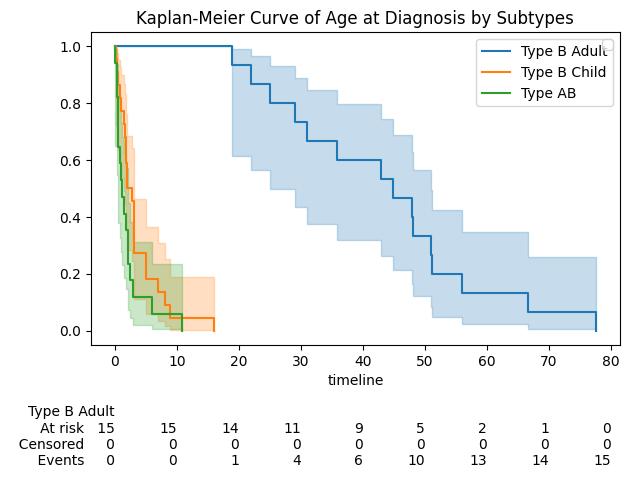
Figure 1. The Kaplan-Meier plot for the three subtypes (Type B Adult, Type B Child, Type AB)
Key observations:
- Type AB and Type B Child are diagnosed early:
- Steep drop in survival curves before age 5
- Most diagnoses occur in early childhood
- Type B Adult experiences delayed diagnosis:
- Gradual decline in survival curve over several decades
- Many are diagnosed in middle age or later
- Subtypes show clear separation:
- Distinct survival curves across groups
- Statistically significant differences confirmed by log-rank test
📈 Statistical Comparison
Conducted a log-rank test to compare survival curves between subtypes and assess whether diagnostic delays differed significantly.
from lifelines import WeibullFitter, ExponentialFitter, LogNormalFitter

models = [
    WeibullFitter().fit(T, E, label="Weibull"),
    ExponentialFitter().fit(T, E, label="Exponential"),
    LogNormalFitter().fit(T, E, label="Log-Normal")
]

fig, ax = plt.subplots()

for model in models:
    model.plot_survival_function(ax=ax)
    aic = model.AIC_
    ax.text(20, 0.8 - 0.1 * models.index(model), f"{model._label} AIC: {aic:.2f}")

plt.title("Model Comparison by AIC")
plt.xlabel("Time since birth (year)")
plt.ylabel("Survival Probability")
plt.tight_layout()
plt.show()
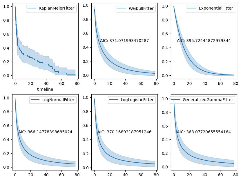
Figure 2. The survival functions overlaid with AIC values.
🧮 Parametric Model Fitting
- Fit various models including Weibull, Log-Normal, Exponential, Log-Logistic, and Generalized Gamma.
- Compared model fit using AIC (Akaike Information Criterion).
- Selected Log-Normal AFT as the best-performing model.
🔍 Prediction by Subtype
- Applied the best model to predict survival (undiagnosed) probability curves for each subtype across a 0–100 year timespan.
- Visualized predictions with subtype-specific curves—helpful for clinicians and researchers interpreting diagnosis timelines.
from lifelines import LogNormalAFTFitter
import numpy as np

lognorm_aft = LogNormalAFTFitter()
lognorm_aft.fit(diagnosis_age_df, duration_col="Time since birth (year)", event_col="Diagnosis")

new_data = pd.DataFrame({"AB": [0, 0, 1], "CH": [0, 1, 0]})
times = np.arange(0, 100, 0.5)

survival_probs = lognorm_aft.predict_survival_function(new_data, times=times)
ax = survival_probs.plot()

ax.legend(["Type B Adult", "Type B Child", "Type AB"])
plt.title("Predicted Survival Curve – Log-Normal AFT")
plt.xlabel("Time since birth (year)")
plt.ylabel("Survival Probability")
plt.show()
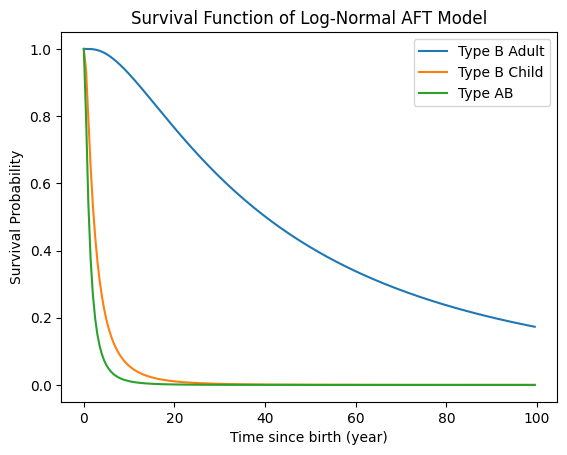
Figure 3. The predicted survival function showing how diagnosis probability changes by subtype.
Findings & Implications
This analysis showed clear differences in time-to-diagnosis across ASMD subtypes. Kaplan-Meier curves revealed that Type AB and childhood-onset Type B patients were diagnosed earlier, while adult-onset Type B cases experienced the longest delays. The Log-Normal AFT model provided the best fit for modeling these differences and enabled prediction of diagnosis probabilities by subtype.
While this example focuses on ASMD, the same survival modeling techniques can be adapted to other rare diseases to quantify diagnostic delays, compare patient subgroups, or support screening research. The methods demonstrated here—handling censored data, fitting multiple survival models, and interpreting time-to-event probabilities—are broadly useful in medical data analysis.
4. Key learning & takeaways
Here are some key lessons I gained while working through this survival analysis project:
What I Learned About Survival Analysis
- There are three major categories of survival models:
- Non-parametric (e.g., Kaplan-Meier): flexible, assumption-free, and good for descriptive analysis
- Parametric (e.g., Weibull, Log-Normal): useful for prediction and interpretation when assumptions are met
- Semi-parametric (e.g., Cox regression): interpretable and flexible for covariates, without requiring full distributional assumptions
- AIC (Akaike Information Criterion) is a valuable tool for selecting the best-fit model among several options.
- When visualizing survival curves with lifelines, it’s helpful to:
- Include 95% confidence intervals to convey uncertainty
- Display at-risk tables to show how many events (diagnoses or censored cases) are observed over time
Practical Challenges and How I Overcame Them
- Survival analysis differs conceptually from typical regression. Grasping its unique assumptions and knowing how to interpret coefficients was essential to making sense of the results.
- Implementing survival models in Python involved trial and error. I relied on:
- lifelines documentation
- Reproducing basic examples
- Experimentation and patience when adapting methods to real-world data, which is often messier than toy examples
Tips for Beginners
- Start with the fundamentals: understand basic statistical concepts and what survival analysis is trying to solve.
- Gain working knowledge of key survival algorithms (Kaplan-Meier, Cox, Log-Normal, etc.).
- Be patient—coding survival models takes attention to detail and a willingness to try, tweak, and retry. Real-world datasets rarely behave like textbook examples, so iteration is part of the process.