How to Reconstruct a Kaplan–Meier Curve from a Published Life Table: A Step-by-Step Beginner’s Guide Using Python
Introduction
In rare-disease research, meta-analyses and systematic reviews often rely on published literature rather than raw individual patient data (IPD). For many analysts new to the field, it’s not immediately obvious that survival curves can still be reconstructed, even when IPD is unavailable.
This tutorial demonstrates how to rebuild a Kaplan-Meier (KM) survival curve from a published life table, step by step. Once the survival function is reconstructed, you can recover meaningful time-to-event insights such as the median time to symptom onset, which is especially valuable for rare diseases where sample sizes are small and reporting formats vary.
What you will learn
By the end of this tutorial, you will understand:
- How to convert a published life table into an estimated Kaplan–Meier survival curve
- How to approximate the number of events in each interval
- How to generate simulated (“pseudo”) individual-level data
- How to fit a KM model in Python using the lifelines package
- How to visualize the survival function and extract median event times
Prerequisites
- Basic familiarity with Python (e.g., using pandas)
- No prior survival-analysis knowledge required
What Is a Life Table, and Why Does It Matter?
Before jumping into code, it’s worth understanding what a life table represents.
A life table reports the number of individuals who remain event-free at specific follow-up times. Even though it does not contain individual observations, it still retains sufficient structure to approximate a survival pattern.
Reconstructing a KM curve from a life table is particularly useful when:
- Only aggregate results are published (common in retrospective cohorts)
- Raw KM curves are missing or provided only as images
- Conducting meta-analyses for rare diseases, where IPD is rarely available
- You need a quantitative estimate of survival metrics (median, percentiles, etc.)
With a bit of algebra and simulation, we can recover a reasonable approximation of the original survival function.
Workflow Overview
To help beginners visualize the full process, here is the conceptual workflow for reconstructing a Kaplan–Meier curve from a life table:
-
Import Python libraries: Load packages for data manipulation (pandas), modeling (lifelines), and visualization (matplotlib).
-
Convert the life-table counts into a DataFrame: Enter (or load) the event-free counts at each follow-up time.
-
Calculate the number of events per interval: Events are approximated using the drop in survival counts between time points.
-
Expand the data into “pseudo” individual-level records: Each row becomes a simulated patient, allowing us to fit a survival model.
-
Fit a Kaplan–Meier model using lifelines.KaplanMeierFitter: Use the simulated data to estimate the survival function.
-
Visualize the KM curve: Plot the reconstructed survival curve to inspect its shape and behavior.
-
Extract key survival metrics: Compute median time to event, percentiles, and other summary statistics.
This workflow provides a practical way to derive time-to-event insights when access to raw patient-level data is limited.
Implementation
Next, I will walk you through the Python code step by step, briefly highlighting the key outputs and how to interpret them.
Steps 3 and 4 are the most important for simulating the Kaplan–Meier function and curve, and are worth particular attention during review.
Step 1: Import Python libraries
import lifelines # Survival analysis library
from lifelines import KaplanMeierFitter # Fit Kaplan-Meier model

import pandas as pd
import numpy as np
import seaborn as sns
import matplotlib.pyplot as plt
Step 2. Convert the life-table counts into a DataFrame
The life table was extracted from a research paper describing the onset of interstitial lung disease (ILD) in a cohort. ILD is a symptom in which lung tissue becomes damaged and cannot fully expand or fill with air.
# Create lifetable DataFrame from given data
data = {
    "year": [0, 1, 2, 3, 4, 5],
    "symptoms_free": [745, 592, 382, 262, 171, 97]
}

df = pd.DataFrame(data)

print(df)
| year | symptoms_free |
|---|---|
| 0 | 745 |
| 1 | 592 |
| 2 | 382 |
| 3 | 262 |
| 4 | 171 |
| 5 | 97 |
The life table reports the number of patients who remained free of the symptom of interest over a follow-up period of up to five years.
It provides the number of patients surviving without ILD from year 1 through year 5, as well as the number at risk at year 0, corresponding to the index date of the retrospective cohort.
Step 3: Calculate the number of events per interval
Next, we need to back-calculate the number of patients who developed the symptom during each time interval.
We assume that no patients were censored and that each individual has a binary status, either with or without the symptom. Under this assumption, the number of events in a given year can be calculated as the difference between the number of symptom-free patients in the previous year and the number of symptom-free patients in the current year.
For example, the number of events in year 1 equals the number of symptom-free patients at year 0 minus the number of symptom-free patients at year 1.
# Compute events per interval (from symptoms_free counts)
df["events"] = df["symptoms_free"].shift(1) - df["symptoms_free"]
df.loc[0, "events"] = 0  # no event at time 0
print(df)
| year | symptoms_free | events |
|---|---|---|
| 0 | 745 | 0 |
| 1 | 592 | 153 |
| 2 | 382 | 210 |
| 3 | 262 | 120 |
| 4 | 171 | 91 |
| 5 | 97 | 74 |
4. Expand the data into “pseudo” individual-level records
Next, we recreate an individual-level dataset that includes each patient’s observed time and symptom-free status, with one row per individual. In this dataset, a value of 1 indicates that the patient developed the symptom, while 0 indicates that the patient remained symptom-free.
# Create expanded individual-level dataset for Kaplan-Meier fitting
records = []
for _, row in df.iterrows():
    year = row["year"]
    events = int(row["events"])
    # event cases
    for i in range(events):
        records.append({"time": year, "event": 1})
for i in range(int(df.iloc[-1]["symptoms_free"])):
    records.append({"time": 5, "event": 0})

df_long = pd.DataFrame(records)
We then verify that the reconstructed dataset contains the correct number of patients at risk (n = 745).
Step 5: Fit a Kaplan–Meier model using lifelines.KaplanMeierFitter
We will fit a Kaplan–Meier function using the reconstructed dataset, applying the KaplanMeierFitter function from the lifelines module.
# Fit Kaplan-Meier model
km = KaplanMeierFitter()
km.fit(durations=df_long["time"], event_observed=df_long["event"])
Step 6: Visualize the KM curve: Plot the reconstructed survival curve to inspect its shape and behavior
# Plot survival function
km.plot_survival_function()

plt.title("Kaplan-Meier Symptom Free Curve")
plt.xlabel("Time (years)")
plt.ylabel("Symptom Free Probability")
plt.ylim(0, 1)
plt.grid()
plt.show()
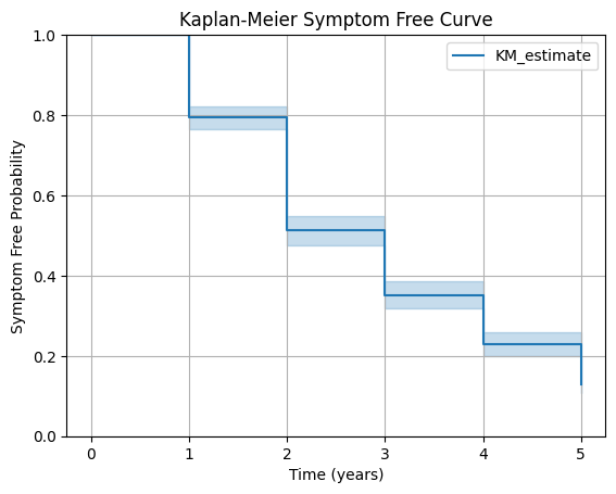
The survival curve illustrates the Kaplan–Meier function from the index year through the end of the follow-up period in the retrospective cohort study.
Each downward step within a time interval reflects the assumption that patients in that interval have a uniform probability of remaining symptom-free.
Step 7: Extract key survival metrics
We are able to obtain the median time to symptom onset directly from the Kaplan–Meier function. This is useful for understanding the overall pattern of symptom development in the cohort.
# Print median survival time
print("Median Symptom Free Time:", km.median_survival_time_)
Method Limitations
While reconstructing a Kaplan–Meier curve from a life table is useful, the approach has several inherent constraints:
- Assumes no censoring: Life tables do not distinguish between events and loss to follow-up. This method treats all declines as events, which may inflate event rates if censoring occurred.
- Assumes uniform timing of events: Events are distributed evenly across each interval, even though real-world data may show clustering that cannot be recovered without individual-level data.
- Not true individual-level data: The expanded dataset matches counts but does not reflect actual patient trajectories. Results should be interpreted as approximations.
- Limited by table granularity: Annual life-table data can only produce annual-level survival patterns. Finer intervals (e.g., monthly) would improve accuracy but are rarely available in published studies.
Final Takeaways
Reconstructing a Kaplan–Meier curve from a life table is far simpler than it initially appears.
With only a few rows of published counts and basic Python code, you can approximate a full survival curve and extract meaningful time-to-event insights.
Here are the key lessons from this guide:
- Life tables contain enough information to rebuild an approximate survival function.
- By computing interval events and expanding them into pseudo–individual-level records, we can fit a KM model without IPD.
- Tools like
lifelinesmake it easy to visualize survival curves and extract median survival time or other summary statistics. - This workflow is especially valuable in systematic reviews, rare disease epidemiology, and health economic modeling, where KM curves are needed but individual-level data are rarely provided.
Overall, this method gives researchers a pragmatic way to extract more value from published evidence, and enables a deeper understanding of survival patterns even when the original dataset is inaccessible.
Download the Full Notebook and Try It Yourself
If you’d like to explore the complete code, visualizations, and step-by-step logic, you can download the full notebook from my GitHub repository.
The notebook includes:
- all Python code used in this tutorial
- expanded comments for beginners
- the reconstructed KM curve
Feel free to adapt the notebook for your own meta-analysis, rare disease research, or health economic modeling projects.