Evaluating Confidence Interval Methods under Skewness: Practical Insights from Simulation
Introduction
Estimating the mean and its confidence interval (CI) is a fundamental task in statistical analysis. Confidence intervals quantify the uncertainty of an estimate, providing a range of plausible values for a population parameter based on sampled data.
However, when data distributions are skewed or overdispersed, standard CI methods may no longer perform reliably:
- They might produce intervals that are too narrow, failing to capture the true mean often enough (under-coverage).
- Or, they might become overly conservative, yielding unnecessarily wide intervals.
This is particularly relevant in fields like healthcare and rare disease research, where data such as hospital length of stay (LOS) commonly exhibit right-skewed distributions with a few extreme outliers. In such cases, choosing an appropriate CI estimation method becomes critical for making valid inferences.
Motivation for Benchmarking Methods
Different methods—such as the t-distribution, z-distribution, and bootstrap percentile approaches—are often used interchangeably for CI estimation. Yet, their performance can vary substantially depending on:
- Sample size
- Data skewness
- Variability (overdispersion)
This project benchmarks these methods under simulated skewed data conditions to evaluate:
- Coverage Probability: How often does the CI contain the true mean?
- Interval Width: How wide is the resulting confidence interval?
The goal is to provide practical insights for analysts working with small, skewed samples, ensuring more reliable and interpretable statistical conclusions.
![]()
Methods
Confidence Interval Estimation Methods
We compared three statistical methods to estimate the 95% confidence interval of the sample mean:
-
t-distribution method
Calculates CI using the sample mean, sample standard deviation, and t-critical value with degrees of freedom (n-1).
-
z-distribution method
Similar to the t-method but uses the normal z-critical value, assuming population standard deviation is known (in practice, sample SD was used).
-
Bootstrap percentile method
Resamples the observed sample with replacement.
The CI is constructed from the 2.5th and 97.5th percentiles of the resampled means.
Simulation of Skewed Data
To benchmark different methods for constructing confidence intervals (CIs) of the mean, we simulated data resembling the distribution of hospital length of stay in autoimmune encephalitis patients. Specifically:
- Data were generated from a log-normal distribution, a typical choice for modeling right-skewed and overdispersed outcomes like hospital stay durations.
- The true mean was set to 20 days, with true standard deviations of 5, 10, 20, and 40 days.
- For each scenario, the corresponding log-space parameters (mu and sigma) were computed to ensure realistic skewness.
- A large population of 10,000 observations was generated per scenario to represent the “true” population.
Simulation Study Design
To evaluate the performance of these methods under varying conditions:
- Sample sizes tested: 10, 30, and 100.
- Skewness levels tested: corresponding to sigma = 0.4, 0.8, and 1.2 in log space.
- For each combination, we repeated the sampling and CI estimation 1,000 times.
Performance Metrics
Two metrics were computed to assess method performance:
- Coverage Probability: Proportion of simulations where the constructed CI contained the true population mean.
- Interval Width: Average length of the confidence intervals across simulations.
Visualization
Bar plots were used to visualize:
- The coverage probabilities of each method relative to the nominal 95% level.
- The average interval widths, illustrating the trade-off between precision and accuracy.
Results
Coverage Probability
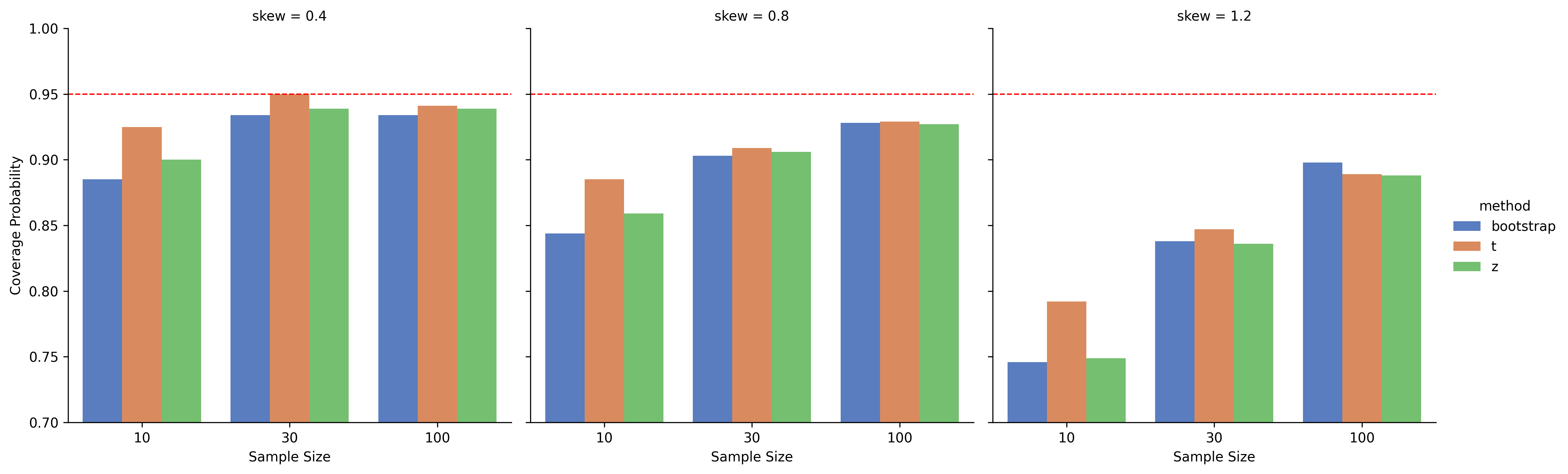
A bar plot comparing the coverage probability of three methods (t-distribution, z-distribution, bootstrap) across:
- Different sample sizes (10, 30, 100)
- Different skewness levels (0.4, 0.8, 1.2)
Interval Width
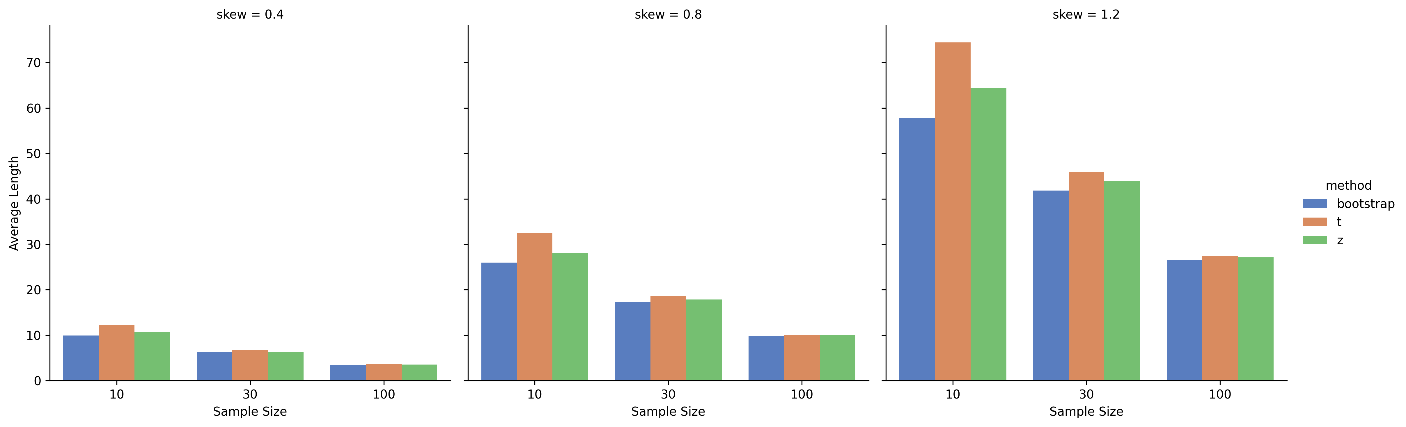
A bar plot comparing the average width (length) of confidence intervals for the same methods, sample sizes, and skew levels.
Discussion
This simulation study compared three common methods—t-distribution, z-distribution, and bootstrap percentile—for constructing 95% confidence intervals (CIs) of the mean in right-skewed, overdispersed data, mimicking hospital length of stay in rare disease contexts.
Key Findings:
- Coverage Probability:
- The t-distribution method consistently provided coverage probabilities closest to the nominal 95% level, even with small sample sizes and increased skewness.
- The bootstrap method, while flexible, showed notable under-coverage in small and highly skewed samples (e.g., <90% for n=10, skew=1.2).
- The z-distribution method tended to under-cover as well, performing worse than t-distribution but slightly better than bootstrap in high skew conditions.
- Interval Width:
- Bootstrap intervals were consistently narrower than those from t- and z-methods, reflecting its efficiency.
- t-distribution intervals were widest, indicating a more conservative approach to uncertainty.
- With larger sample sizes (n=100), the differences in interval width narrowed, and all methods performed better.
Interpretation:
These results highlight a bias-variance trade-off:
- Bootstrap offers more precise (narrower) intervals but at the cost of coverage reliability, especially in small, skewed samples.
- t-distribution sacrifices precision (wider intervals) to maintain more accurate coverage.
- z-distribution is suboptimal when sample sizes are small and data is skewed, as it assumes normality which is not met.
Practical Implications:
- For small sample studies with skewed data (common in rare disease research), the t-distribution method is safer for mean estimation, despite its conservatism.
- Bootstrap methods should be applied cautiously when sample size is limited or data is heavily skewed.
- With larger samples, all methods converge in performance, making bootstrap’s efficiency more appealing.
🧑💻 Code Snippets
To help you apply these methods in your own analysis, here are reusable Python code snippets for constructing confidence intervals (CIs) of the mean using t-distribution, z-distribution, and bootstrap methods. These functions are included in the full Jupyter notebook for reproducibility.
📏 t-distribution Confidence Interval
from scipy import stats
import numpy as np

def ci_t(sample):
	n = len(sample)
	m = np.mean(sample)
	se = np.std(sample, ddof=1) / np.sqrt(n)
	t_crit = stats.t.ppf(0.975, df=n-1)
	return m - t_crit * se, m + t_crit * sedef ci_t(sample, ci_level=0.95):
	    """Compute t-distribution confidence interval for the sample mean."""
	    n = len(sample)
	    sample_mean = np.mean(sample)
	    sample_se = np.std(sample, ddof=1) / np.sqrt(n)
	    t_crit = stats.t.ppf(0.5 + ci_level / 2, df=n-1)
	    lower = sample_mean - t_crit * sample_se
	    upper = sample_mean + t_crit * sample_se
	    return lower, upper
📏 z-distribution Confidence Interval
def ci_z(sample):
    n = len(sample)
    m = np.mean(sample)
    se = np.std(sample, ddof=1) / np.sqrt(n)
    z_crit = stats.norm.ppf(0.975)
    return m - z_crit * se, m + z_crit * se
🔁 Bootstrap Percentile Confidence Interval
def ci_bootstrap(sample, n_bootstraps=1000, ci=0.95):
    n = len(sample)
    means = []

    for _ in range(n_bootstraps):
        resample = np.random.choice(sample, size=n, replace=True)
        means.append(np.mean(resample))

    alpha = 1 - ci
    lower = np.percentile(means, 100 * (alpha / 2))
    upper = np.percentile(means, 100 * (1 - alpha / 2))
    return lower, upper
📝 How to Use:
# Example usage with your sample data:
sample_data = np.random.lognormal(mean=np.log(20), sigma=0.8, size=30)

t_ci = ci_t(sample_data)
z_ci = ci_z(sample_data)
bootstrap_ci = ci_bootstrap(sample_data, n_bootstraps=1000)

print(f"t-distribution CI: {t_ci}")
print(f"z-distribution CI: {z_ci}")
print(f"Bootstrap CI: {bootstrap_ci}")
🔗 Full Notebook & Reproducibility
For full simulation workflows, including population data generation, performance metrics, and visualization:
👉 View the Jupyter Notebook on GitHub
Or, view the notebook on Binder with no installing dependencies ![]()