A Beginner’s Hands-On Guide to Meta-Analysis and Confidence Intervals
Introduction
This post serves as a hands-on tutorial for beginners who are learning how to conduct meta-analysis in the context of microbiome research. Whether you’re synthesizing findings from multiple studies or comparing gut microbiome diversity across populations, this guide is designed to help you get started with clarity and confidence.
What You’ll Gain from This Tutorial
- Clear, minimal explanations of key concepts in fixed-effect and random-effects meta-analysis—no prior advanced statistics required
- Reusable R code snippets using the well-documented meta package, making it easy to apply the methods to your own dataset
- Practical guidance on choosing appropriate models, weighting strategies, and confidence interval methods, tailored to common challenges in microbiome data
Whether you’re a graduate student, postdoc, or early-career researcher, this tutorial will help you bridge the gap between statistical theory and real-world implementation—so you can focus on the biological insights that matter.
What You Need to Know First
1. Weighting: Parametric vs. Non-parametric Approaches
The goal of meta-analysis is to synthesize findings across studies to estimate a single pooled effect size (e.g., odds ratio, risk difference, mean difference).
Since not all studies are equally informative, each study is assigned a weight that determines its contribution to the pooled estimate.
Two common approaches to weighting:
- Sample size–based weighting (non-parametric): Larger studies receive more weight based solely on their sample sizes. This approach is simpler but does not account for the variability in effect size estimates.
- Inverse-variance weighting (parametric): Weights are assigned as the inverse of the variance of each study’s effect size. This method prioritizes more precise studies and is the basis for most modern meta-analytic models.
2. Fixed vs. Random Effects Models and Their Assumptions
Meta-analysis models differ in how they conceptualize the true effect:
- Fixed-effect model assumes all studies estimate the same true effect size. Differences between studies arise only due to sampling error.
- Random-effects model assumes that each study estimates a different (yet related) true effect size. Differences reflect both within-study variance (sampling error) and between-study heterogeneity (true variation in effects).
The fixed-effect model is appropriate when studies are highly similar (homogeneous), while the random-effects model is more flexible and widely used when heterogeneity exists.
3. Between-study Heterogeneity (τ²)
Between-study heterogeneity reflects real differences in effect sizes due to factors like study population, intervention, or setting.
In a random-effects model, this variability is quantified by τ² (tau-squared).
Several estimators are available to compute τ², including:
- DerSimonian–Laird (DL) – the most commonly used.
- Restricted Maximum Likelihood (REML) – more accurate in small samples.
- Paule–Mandel, Empirical Bayes, etc.
4. 95% Confidence Interval of the Pooled Effect
The 95% confidence interval (CI) around the pooled effect size represents the uncertainty of the estimate — that is, the range in which the true effect is expected to lie 95% of the time.
For fixed-effect models, the CI is narrower because only sampling error is considered.
For random-effects models, the CI is wider due to the inclusion of between-study heterogeneity (τ²).
Methods to compute CIs include:
- Normal approximation (Wald-type) – common default.
- Knapp–Hartung adjustment – improves coverage in random-effects models, especially with few studies.
Step-by-Step Guide
This section introduces two common approaches to synthesizing study results in meta-analysis: the fixed-effect modeland the random-effects model. A guiding question is: Do we assume that all studies estimate a single true effect size? If yes, use a fixed-effect model; if not, or if there is heterogeneity, use a random-effects model.
Fixed-Effect Model
Step 1: Calculate Effect Sizes for Individual Studies
At the first place, we calculate the effect size for each study included in the meta-analysis. Effect size quantifies the strength of a difference or relationship between variables. Common types include mean difference, standardized mean difference, odds ratio, and correlation.
Step 2: Assign Weights
To account for how much each study contributes to the overall effect estimate, we assign weights to each study.
There are two common approaches:
a) Sample Size–Based Weighting
Each study is weighted according to its sample size:
\[w_i = n_i\]where \(n_i\) is the sample size of study \(i\).
We may also use normalized weights or w̃_i:
\[w̃_i = n_i / ∑n_i\]This approach is simple while it does not account for differences in measurement precision across studies.
b) Variance-based Weighting
A more statistically rigorous method is to weight each study inversely proportional to the variance of its effect size estimate:
\[w_i = 1 / v_i\]where \(v_i\) is the estimated variance of the effect size \(x_i\) from study \(i\).
- This approach gives greater weight to more precise studies (those with smaller variances).
- It is the standard method used in most fixed-effect meta-analysis.
- In practice, the variance v_i is often derived from standard errors, confidence intervals, or reported summary statistics.
| Effect Size Type | Variance Formula (\(v_i\)) |
|---|---|
| Mean Difference (2 groups) | \(v_i = (SD₁² / n₁) + (SD₂² / n₂)\) |
| Standardized Mean Difference (SMD) | \(v_i = (n₁ + n₂)/(n₁ × n₂) + d²/(2 × (n₁ + n₂))\) |
| Single Group Mean | \(v_i = SD² / n\) |
Step 3: Calculate the Weighted Mean Effect Size
The overall pooled effect size under the fixed-effect model is computed as:
\[μ* = ∑(w_i × x_i) / ∑w_i\]where x_i is the effect size estimate from study i, and w_i is its assigned weight.
Step 4: Estimate the Variance of the Weighted Mean
Assuming a fixed-effect model and using inverse-variance weights or sample-size weights, the variance of the pooled effect is estimated as:
\[Var(μ*) = 1 / ∑w_i\]Step 5: Calculate the Standard Error
The standard error (SE) of the pooled effect size is the square root of its variance:
\[SE = √Var(μ*)\]Step 6: Compute the 95% Confidence Interval
Using the normal (Z) distribution, the 95% confidence interval for the pooled effect size is:
\[μ* ± 1.96 × SE\]Here, the critical value, Z-score 1.96 leaves 97.5% of the standard normal distribution (mean = 0, SD = 1) to the left of it.
Random Effects Models
Random-effects models account for the possibility that true effect sizes differ across studies, acknowledging heterogeneity beyond sampling error.
Step 1: Test for Heterogeneity
We calculate the Q statistic to test for heterogeneity among studies:
\[Q = ∑ w_i^FE × (x_i − μ*_FE)²\]where w_i^FE is fixed-effect weights, μ*_FE is fixed-effect pooled mean
A large Q indicates substantial between-study heterogeneity—meaning real differences in effect sizes may exist.
The Higgins & Thompson’s I², derived from Q, is an alternative metric that quantifies the percentage of variation due to heterogeneity rather than chance.
Step 2: Estimate the Between-Study Variance (τ²)
We now estimate how much true effects differ between studies - this variability is called between-study variance, or τ².
Several estimators are available:
- DL (DerSimonian and Laird) - a widely used default method
- ML (Maximum Likelihood)
- REML (Restricted Maximum Likelihood)
These methods differ in how they estimate uncertainty, especially in small samples.
Step 3: Determine Random-Effects Weights
Each study is now weighted based on both within-study variance and between-study variance:
\[w_i = 1 / (v_i + τ²)\]where v_i: within-study variance, and τ²: between-study variance
This formula reflects a study with less precision and higher heterogeneity dataset gets less weight.
Step 4: Calculate the Random-Effects Weighted Mean
We then pool the study effect size using a weighted average:
\[μ* = ∑ (w_i × x_i) / ∑ w_i\]This gives a more generalizable average effect across varying study contexts.
Step 5: Calculate the Standard Error
The uncertainty around the pooled effect size is estimated by:
\[SE = √(1 / ∑ w_i)\]This SE will be larger than under the fixed-effect model due to added uncertainty from heterogeneity.
Step 6: Choose a Confidence Interval Method
There are multiple options for calculating the 95% confidence interval around the pooled estimate in random-effects models:
a) z-distribution Method
- Assumes a normal distribution
- Does not adjust for uncertainty in estimating τ²
b) t-distribution Method
- Uses the t-distribution with k−1 degrees of freedom
- Accounts for small-sample (n < 30) uncertainty better than the z-method
c) Hartung-Knapp (HK) Method
This method gives wider but more reliable intervals, especially when the number of studies is small or heterogeneity is high.
First, calculate the improved variance estimate:
\[Var_w(μ*) = ∑ w_i × (x_i − μ*)² / [(k − 1) × ∑ w_i]\]Then, construct the confidence interval:
\[CI = μ* ± t_(k−1, 1−α/2) × √Var_w(μ*)\]Flowchart Overview
The flowchart below visually summarizes the critical steps involved in conducting a meta-analysis using either a fixed-effect or a random-effects model. It is designed to help readers quickly grasp the overall workflow and key distinctions between the two approaches.
- Decision points appear at the top, guiding model selection based on assumptions about study heterogeneity.
- Color coding is used to clearly distinguish the fixed-effect pathway from the random-effects pathway.
- Dashed lines highlight key outcome variables at each stage (e.g., pooled effect size, standard error, confidence intervals).
- Steps flow logically from calculating individual effect sizes to pooling, estimating uncertainty, and reporting the final results.
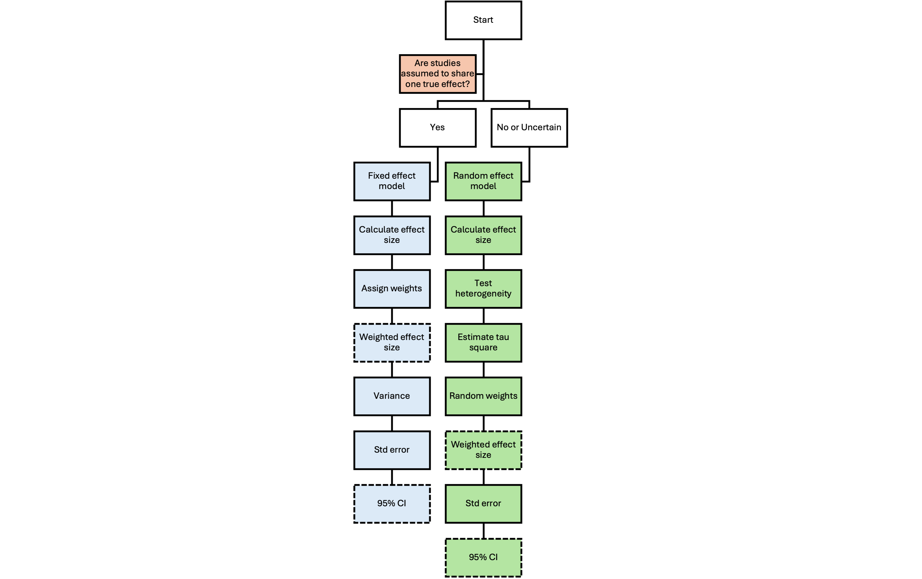
This diagram complements the written walkthrough by providing a high-level visual guide to the computational and statistical logic behind each model type.
Easy R Steps for Meta-Analysis
Example Dataset
To make the code examples more practical and relevant to microbiome researchers, this post uses a real dataset from a published meta-analysis on the impact of exclusive breastfeeding on infant gut microbiome diversity.
The data were drawn from high-quality, peer-reviewed studies, including contributions from respected researchers such as Dr. Louise Kuhn and Dr. Anita Kozyrskyj, who kindly shared accessible summary statistics and metadata. Dr. Kozyrskyj was also my supervisor during my postdoctoral fellowship, and her support made it possible to reproduce this meta-analysis for educational purposes.
The dataset below includes:
- Study reference
- Sample size
- Effect size (diversity difference)
- Standard error of the effect size
Notably, the Subramanian et al. study (conducted in Bangladesh) had the largest sample size and therefore the highest precision (i.e., lowest standard error), contributing significantly to the meta-analysis.
| Study | Sample Size | Diversity Diff. | SE |
|---|---|---|---|
| Subramanian et al., 2014 (Bangladesh) | 322 | 0.26 | 0.0718 |
| Azad et al., 2015 (Canada) | 167 | 0.33 | 0.1583 |
| Bender et al., 2016 (Haiti) | 48 | -0.11 | 0.3474 |
| Wood et al., 2018 (South Africa) | 143 | 0.31 | 0.2235 |
| Pannaraj et al., 2017 (USA(CA/FL)) | 230 | 0.37 | 0.1492 |
| Sordillo et al., 2017 (USA(CA/MA/MO)) | 220 | 0.77 | 0.1971 |
| Thompson et al., 2015 (USA(NC)) | 21 | 0.3 | 0.4239 |
Computational Tools
To support reproducibility and hands-on learning, this use case provides re-usable R code snippets that implement two essential steps in a typical microbiome meta-analysis:
- Fixed-effect and random-effects models using inverse-variance weighting
- Forest plot visualization of individual and pooled study results
After a brief comparison of available tools, the R ecosystem was chosen over Python due to its more mature, stable, and flexible support for meta-analysis, especially in microbiome and clinical research contexts.
The analysis was implemented using the meta R package, which is:
- Well-documented and actively maintained
- Supported by detailed tutorials and vignettes
- Beginner-friendly, yet robust enough for advanced use
# Perform fixed-effect and random-effect models on diversity difference using inverse variance
weightmicrobiome_sdd = meta::metagen(TE = diversity_diff, # Study effect size
                                    seTE = se, # Standard error of effect sizes
                                    studlab = study, # Study labels
                                    data = microbiome_df, # Data frame containing statistical information
                                    common = TRUE, # Conduct fixed-effect model meta-analysis
                                    random = TRUE, # Conduct random-effect model meta-analysis
                                    prediction = FALSE, # Not print prediction interval
                                    method.I2 = "Q", # Method used to estimate heterogeneity statistics I^2
                                    method.tau = "DL", # DerSimonian-Laird estimator
                                    method.tau.ci = "J", # Method by Jackson (2013)
                                    method.random.ci = "HK" # Method by Hartung and Knapp (2001a/b)
                                    )
Understanding key arguments in meta::metagen()
To support beginners who may have only basic familiarity with meta-analysis, each function in this post includes annotated explanations of its core arguments. In particular, the R function meta::metagen()—used to compute fixed- and random-effects models—contains several powerful arguments that greatly increase its flexibility.
Among these, four arguments stand out as especially important:
- method.I2 – Controls how the I² statistic (a measure of heterogeneity) is calculated.
- method.tau – Specifies the method for estimating the between-study variance (τ²), such as DerSimonian-Laird, REML, or ML.
- method.tau.ci – Determines how the confidence interval for τ² is calculated.
- method.random.ci – Selects the method used to calculate the confidence interval around the random-effects pooled estimate (e.g., classical vs. Hartung-Knapp).
These arguments offer flexibility and customization, especially when tailoring the analysis to match study heterogeneity or small-sample concerns. However, intentional use requires a solid understanding of their conceptual foundations.
The earlier sections of this post walk through these core concepts to help you build the minimal understanding needed to make informed choices.
For a deeper dive and full list of options, consult the official documentation of the meta package. Exploring these arguments will help you fully leverage the power of metagen() in your own microbiome meta-analyses.
summary(microbiome_sdd)
                          95%-CI           %W(common)  %W(random)
Subramanian et al., 2014 (Bangladesh)   0.2600 [ 0.1193; 0.4007]    57.3       40.7
Azad et al., 2015 (Canada)              0.3300 [ 0.0197; 0.6403]    11.8       15.7
Bender et al., 2016 (Haiti)            -0.1100 [-0.7909; 0.5709]     2.4        4.0
Wood et al., 2018 (South Africa)        0.3100 [-0.1281; 0.7481]     5.9        8.9
Pannaraj et al., 2017 (USA(CA/FL))      0.3700 [ 0.0776; 0.6624]    13.3       17.1
Sordillo et al., 2017 (USA(CA/MA/MO))   0.7700 [ 0.3837; 1.1563]     7.6       11.0
Thompson et al., 2015 (USA(NC))         0.3000 [-0.5308; 1.1308]     1.6        2.7

Number of studies: k = 7

                         95%-CI                   z|t     p-value
Common effect model:     0.3162 [0.2097; 0.4227]   5.82   < 0.0001
Random effects model:    0.3367 [0.1602; 0.5132]   4.67     0.0034

Quantifying heterogeneity (with 95%-CIs):
tau^2 = 0.0073 [0.0000; 0.2032]; tau = 0.0855 [0.0000; 0.4508]
I^2 = 20.6% [0.0%; 64.0%]; H = 1.12 [1.00; 1.67]

Test of heterogeneity:
Q = 7.56, df = 6, p-value = 0.2723

Details of meta-analysis methods:
- Inverse variance method
- DerSimonian-Laird estimator for tau^2
- Jackson method for CI of tau^2 and tau
- I^2 calculation based on Q
- Hartung-Knapp adjustment for random effects model (df = 6)
Draw forest plot
png(file = "forestplot.png", height = 800, width = 1200)

meta::forest(microbiome_sdd,
            sortvar = TE, # Sort study by effect sizes in increasing order
            prediction = FALSE, # Not show prediction interval
            leftcols = c("study", "sample_size", "diversity_diff", "se"),
            leftlabs = c("Study", "Sample Size", "Diversity Diff.", "SE"),
            print.tau2 = TRUE)

dev.off()
Interpret the Forest Plot
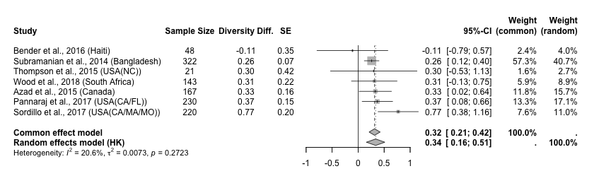
This forest plot compares the results of seven studies evaluating gut microbiome diversity difference (DD) between groups. It shows both individual study results and pooled estimates under fixed-effect and random-effects models.
1. Study Data (Left Side)
- Each row corresponds to a single study included in the meta-analysis.
- DD stands for diversity difference, which is the effect size used in this analysis.
- SE stands for standard error, which reflects the precision of the effect size estimate. Smaller SE means higher precision.
2. Confidence Intervals and Visual Elements (Middle Area)
- Horizontal lines show the 95% confidence interval (CI) for each study’s effect size.
- Squares represent the point estimate of each study. Larger squares indicate greater weight in the analysis.
- The vertical solid line at 0 is the line of no effect—values to the right suggest a positive effect.
- Diamond shapes summarize the pooled effect estimates:
- The gray diamond: fixed-effect (common-effect) model
- The white diamond: random-effects model
- The red horizontal bar under the diamond is the prediction interval, indicating the likely range of effect sizes in future studies.
3. Result Summary (Right Side)
- The 95% CI for each study shows the uncertainty around its effect estimate.
- The columns Weight (common) and Weight (random) show how much each study contributes to the respective model.
- In the fixed-effect model, Study 1 carries 57.3% of the weight due to its very low SE (high precision).
- In the random-effects model, weights are more evenly distributed because the model also accounts for between-study heterogeneity (τ²).
4. Heterogeneity (Bottom Statistics)
- I² = 20.6%: Indicates low to moderate heterogeneity—i.e., some variation in effect sizes across studies, but not extreme.
- p = 0.2723: The test for heterogeneity is not statistically significant, meaning we cannot reject the idea that all studies may share one common effect size.
Summary Interpretation
- The pooled effect sizes from the fixed-effect model (0.32) and the random-effects model (0.33) are very similar, which suggests that the result is robust and stable.
- Since mild heterogeneity is present, the random-effects model is more appropriate for generalization.
- The prediction interval [0.09, 0.57] suggests that future studies are still likely to show a positive effect, though the effect size may vary in strength.
Practical Recommendations
Fixed-Effects Models: Use the standard z-distribution method with size-weighted means when the number of studies is large.
Random-Effects Models: Prefer the weighted variance confidence interval, such as HK, method for better coverage and less sensitive to which estimator used for τ².
Sample Size Weighting is appropriate when:
- Variance estimates are unavailable or unreliable
- Interpretability is a priority
- Study precisions are comparable
Best Practice: Report both parametric and nonparametric weighted results to test the robustness of conclusions.
References
- Perplexity research report
- Doing meta-analysis in R Chapter 3-6