From Practice to Framework: Reusable PSA Tools for Cost-Effectiveness and Epidemiology Modelling
Background
This article is intended to share practical learning and hands-on experience with probabilistic sensitivity analysis (PSA), drawn from real-world health-economic work in rare-disease therapy.
It provides a walkthrough of a reusable PSA architecture, illustrated with use cases, and introduces a probability-distribution inventory with a quick-selection guide for choosing appropriate distributions in PSA. Although the examples come from one working project, the framework is broadly applicable to cost-effectiveness and epidemiology modelling projects that require sensitivity analysis.
The article focuses on the applied aspects of PSA, how to use statistical probability distributions, Excel’s built-in formulas, and backend VBA to implement simulations. It intentionally does not cover the theoretical foundations of statistical distributions or general Excel functionality, which are beyond its intended scope.
Conceptual workflow for implementing uncertainty simulation in PSA
Problem and Solution
The primary goal of PSA is to quantify how uncertainty in model inputs affects the outputs of a cost-effectiveness (CE) model. PSA uses statistical simulation, typically Monte Carlo simulation, to generate thousands of model runs, each drawing inputs from predefined, plausible uncertainty ranges.
From my learning and real-world project experience, two steps are often the most challenging when implementing PSA in Excel:
- building a robust PSA architecture (in-cell formulas and VBA), and
- selecting appropriate probability distributions for each input parameter.
To address these challenges, I’ve developed a set of reusable PSA tools designed to make these steps easier and more consistent across projects.
Conceptual Workflow
The high-level workflow for PSA includes:
- Select an appropriate probability distribution
- Retrieve deterministic inputs and standard deviations from references
- Parameterize the selected distribution
- Generate random samples
- Run the simulation
The following sections walk through the architecture and each step in more detail.
Introduction to two reusable tools
First Tool: PSA Architecture in Excel
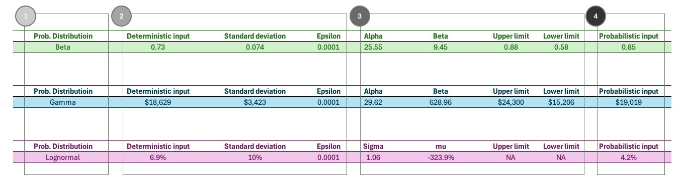
The screenshot below illustrates the main PSA architecture in Excel, with four framed sections corresponding to the first four steps of the PSA workflow.
I’ve also uploaded the Excel workbook containing this PSA setup for anyone interested in reviewing or applying it. Please refer to the “Generate_uncertainty” sheet for the full implementation.
In brief, the visible portion of the PSA architecture includes four components:
- Selection of probability-distribution types
- Entry of deterministic inputs and standard deviations
- Parameterization of the chosen distribution
- Setup for generating random samples
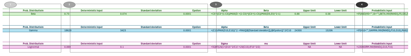
The hidden portion contains reusable in-cell formulas that calculate distribution parameters and generate uncertainty-adjusted random inputs. These formulas support consistent and transparent PSA implementation across projects.
The Second Tool: Probability-Distribution Inventory
Choosing an appropriate probability distribution for each model input is the first and most critical step in PSA.
As demonstrated in the ISPOR good practice guidelines for uncertainty analysis, high-quality research requires selecting probability distributions that appropriately reflect the nature of the data being modeled. The guidelines also provide practical recommendations for choosing distributions tailored to different data types. The full paper is available here.
This selection requires both an understanding of statistical distributions and domain knowledge in health economics or epidemiology.
The inventory provides the key information needed to make informed decisions, including:
- the support (range) of each distribution,
- parameterization details,
- example use cases, and
- links to external references for further reading.
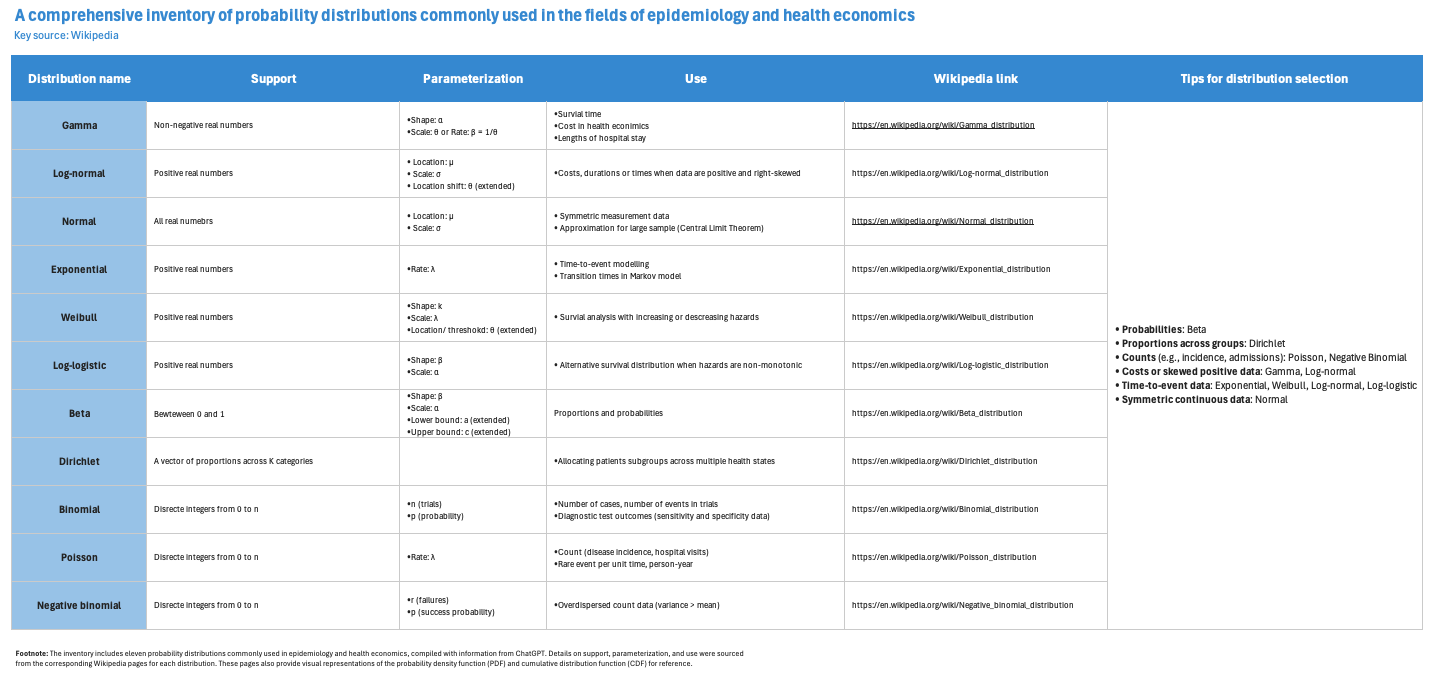
The rightmost column also includes practical tips to support distribution selection in real-world modelling.
A later section of this article will explain how to use this inventory more effectively.
End-to-end walkthrough of the Excel-based PSA architecture
As illustrated in Figure 1, this section walks through the four key PSA steps implemented in Excel, followed by an overview of the simulation-validation process and the dashboard used to visually inspect the results.
Steps (corresponding to the four framed sections)
- Select an appropriate probability distribution
- Choose a suitable distribution for the parameter of interest. Refer to the Inventory sheet for guidance.
- This choice is critical because it determines the required parameterization.
- For demonstration, the sheet highlights three commonly used distributions: Beta, Gamma, and Lognormal.
- Enter deterministic inputs, standard deviation, and optional epsilon
- Input the deterministic value (e.g., the mean) and its standard deviation, typically sourced from literature such as ICER (2019).
- An optional epsilon (e.g., 0.0001) can be used when the standard deviation is reported as zero; it is not needed when a non-zero SD is available.
- Parameterize the selected distribution
- The model automatically calculates the required distribution parameters (e.g., Alpha, Beta, Mu, Sigma) using built-in formulas.
- Optional upper and lower limits may be entered when reported in the literature.
- Parameterization uses the previously entered mean, standard deviation, and, if applicable, epsilon.
- Generate random samples
Column J contains formulas that generate random samples based on the chosen distribution and its parameterization.
Running the simulation
To test the setup:
- Go to the Validate_simulation sheet
- Click Run simulation
- Clear previous simulation results if needed
The buttons are linked to established backend VBA.
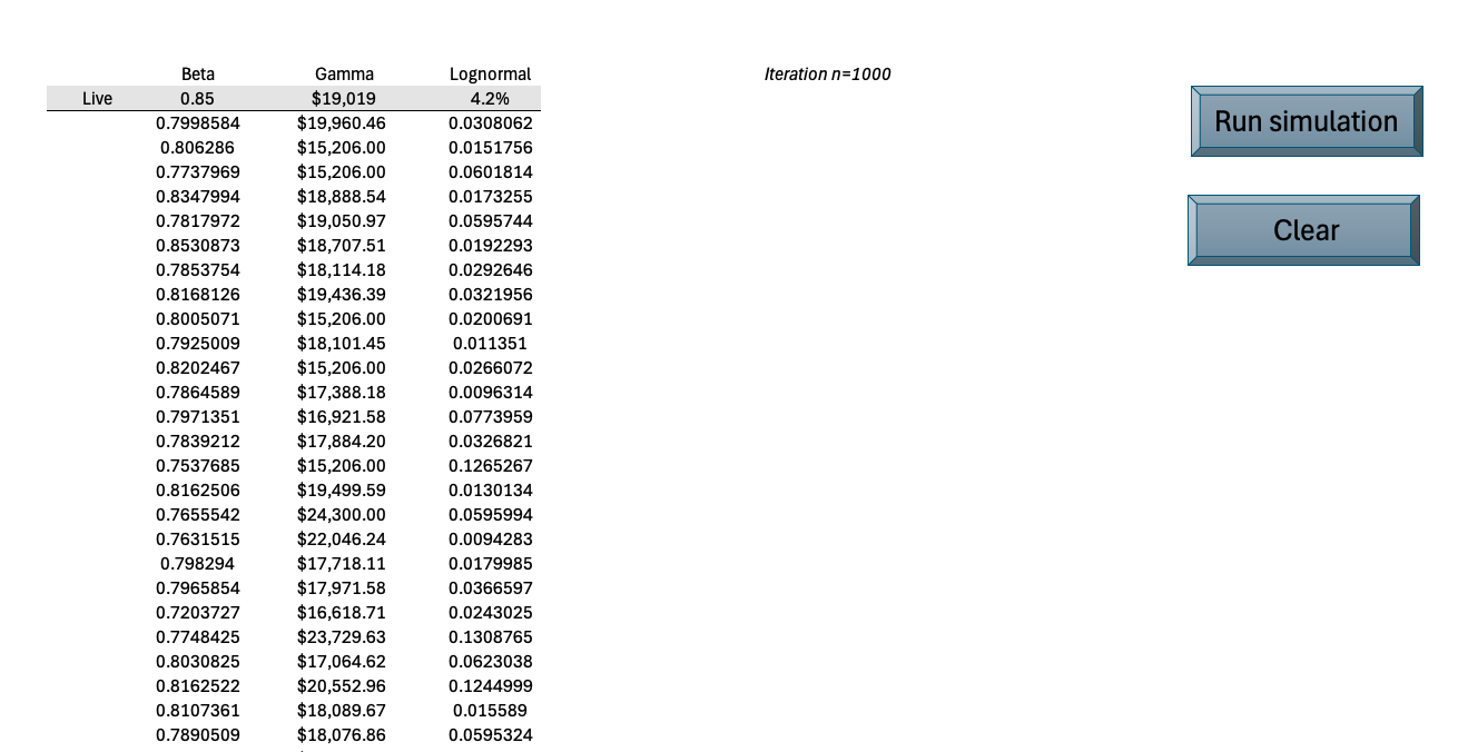
Briefly, the Live row displays probability outputs for the current iteration (referencing the previous sheet), while the rows below it store results from all 1,000 iterations. Two user-friendly buttons on the right allow users to run or clear the backend VBA simulations.
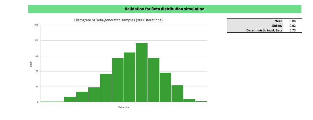
The Dashboard supports visual inspection of the simulation outputs. The histogram displays the distribution of randomly sampled values for the selected probability distribution, while the framed summary table on the right compares the mean and standard deviation of the sampled data against the deterministic inputs.
How to use the probability-distribution inventory
As shown in Figure 3, users can begin with column “Tips for distribution selection” to quickly narrow down candidate probability distributions that align with the characteristics of the HE or Epi parameter of interest. From there, users can review essential properties of each candidate distribution, such as whether its support matches the actual range of the model input, and whether relevant use cases exist. The parameterization section and linked Wikipedia references provide additional guidance for implementing the distribution statistically.
Conclusion
The two tools introduced here are designed to support users in implementing PSA in Excel through a reusable architecture, clear documentation, VBA-powered simulations, and intuitive visual inspection tools.
The PSA architecture can be integrated into nearly any CE modelling project with only minor adjustments. The VBA scripts are also adaptable to other projects with minimal modifications.
The probability-distribution inventory, along with its practical selection guide, helps users choose appropriate distributions for each model input with confidence.
Excel file on Github
If you’re interested in exploring or applying these tools, you can download the macro-enabled Excel workbook, “PSA_Implementation_Tools_2025.11.24_DZ.xlsm,” from my GitHub repository (here).