How to Reconstruct Disease Onset Age Distributions Using Summary Statistics: A Rare Disease Use Case in Python
In rare disease research, one of the most frustrating barriers is the lack of individual-level data. While disease onset age is critical for modeling epidemiological burden and designing trials, most published studies only report summary statistics like medians or quartiles.
But what if you could reconstruct a full onset age distribution from just these summary stats?
In this post, I’ll walk you through how to simulate granular age-at-onset profiles using Python. We’ll use anti-GABABR autoimmune encephalitis (AIE) as a real-world example and fit three candidate distributions—log-normal, Weibull, and generalized gamma—using a technique called quantile matching.
You’ll learn how to:
- Fit distributions to summary statistics using constrained optimization
- Simulate individual-level onset ages
- Compare model fit across distributions
- Estimate age-band proportions with bootstrap confidence intervals
Whether you’re working on a burden-of-disease model, HTA submission, or just exploring rare disease analytics, this post will give you a reproducible template to start from.
The reusable Python notebook is available at here
Step 1: Background and Input Data
Our example comes from Lamblin et al. (2024), who reported onset age statistics for anti-GABABR AIE:
median = 66
q1 = 61
q3 = 72
min = 19
max = 88
mean = 67
size = 111
For our modeling, we’ll focus on the three quantiles (Q1, median, Q3).
Step 2: Quantile Matching to Fit Distributions
We’ll use constrained optimization to find the best-fitting parameters such that theoretical quantiles match the reported ones.
Here’s the objective function for a log-normal distribution:
from scipy.stats import lognorm
from scipy.optimize import minimize
import numpy as np

# Empirical quantiles
empirical_q = [61, 66, 72]

# Objective function: Minimize squared differences between model and empirical quantiles
def objective(params):
    mu, sigma = params
    if sigma <= 0:
        return np.inf
    dist = lognorm(s=sigma, scale=np.exp(mu))
    theo_q = dist.ppf([0.25, 0.5, 0.75])
    return np.sum((np.array(theo_q) - empirical_q)**2)

# Initial guess for mu and sigma
initial_guess = [np.log(66), 0.5]

# Optimize
result = minimize(objective, x0=initial_guess, bounds=[(0, None), (0.01, 5)])

mu_fit, sigma_fit = result.x
Fitted parameters:
- μ (log-scale mean): 4.192
- σ (log-scale SD): 0.123
This defines the objective function for optimization:
- Takes parameters mu and sigma as input
- Returns infinity if sigma is non-positive (constraint)
- Calculates theoretical quantiles using the log-normal distribution with given parameters
- Returns the sum of squared differences between theoretical and empirical quantiles (this is what we want to minimize)
We repeat this process for Weibull and generalized gamma as well.
Step 3: Visualizing the Simulated Distribution
Once we’ve fitted the distribution, we simulate 10,000 onset ages and plot:
- Left: Histogram of simulated ages
- Right: CDF overlay comparing empirical and model quantiles
Example output for log-normal:
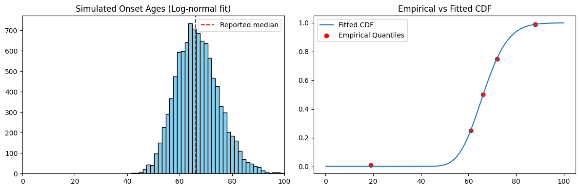
This dual-panel visualization helps assess how well the simulated distribution captures the shape and tails of the reported data.
Step 4: Comparing Goodness-of-Fit
We assess fit using the sum of squared differences between simulated and empirical quantiles:
| Distribution | Sum of Squared Errors |
|---|---|
| Log-normal | 0.0916 |
| Weibull | 0.5238 |
| Generalized Gamma | 0.0772 (best fit) |
Unsurprisingly, the generalized gamma distribution—known for its flexibility—performed best.
Step 5: Estimating Age-Band Proportions with Bootstrap CI
Let’s say we want to estimate the proportion of patients in three age bands:
- <12 years
- 12–17 years
- ≥18 years
We use bootstrapping (1,000 iterations) to estimate proportions and their 95% confidence intervals:
age_bands = [(0,12), (12,18), (18,100)]
n_iterations = 1000
n_samples = 10000

from scipy.stats import gengamma

# Using best-fit generalized gamma parameters
bootstrap_results = []
for _ in range(n_iterations):
    sim_ages = gengamma(a=26.611, c=1.583, scale=8.409).rvs(n_samples)
    proportions = [np.mean((sim_ages >= low) & (sim_ages < high)) for (low, high) in age_bands]
    bootstrap_results.append(proportions)
Resulting summary:
| Age Band | Mean Proportion | 95% CI Lower | 95% CI Upper |
|---|---|---|---|
| 0–12 | 0.0000 | 0.0000 | 0.0000 |
| 12–18 | 0.0000 | 0.0000 | 0.0000 |
| 18+ | 0.9999 | 0.9997 | 1.0000 |
Visualization:
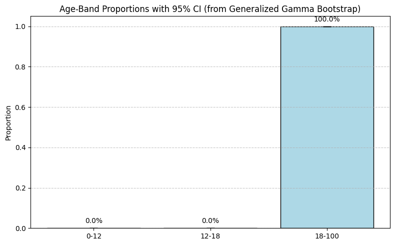
This clearly shows the distribution is concentrated in adult-onset.
Conclusion and Reuse
This method allows you to simulate realistic onset age distributions using only summary statistics. It’s particularly valuable in rare disease modeling, where raw data are scarce but precise modeling inputs are needed.
You can adapt this notebook by:
- Swapping in new quantiles from another disease or study
- Testing additional distribution families (e.g., skew-normal)
- Extending to model time to diagnosis or treatment delay
Whether you’re building HTA models or conducting evidence synthesis, this is a scalable, data-light, and transparent tool to add to your workflow.