Parametric Survival Fit & PSA for Age-at-Onset in Autoimmune Disease: Generalized Gamma Workflow
In rare disease epidemiology, researchers often face a familiar challenge: most published studies do not provide individual-level patient data. Instead, they report only high-level summary statistics such as quartiles, means, and total sample size. Yet for health economic modeling, burden of disease estimation, or natural history modeling, we still need to understand the full age-at-onset distribution, including its shape, skew, and uncertainty.
This article presents a practical workflow for reconstructing that distribution using parametric survival models, with a focus on the generalized gamma distribution. We will also show how to incorporate parameter uncertainty using probabilistic sensitivity analysis (PSA) and how to compute key outputs such as diagnosis probabilities within specific age bands.
This workflow is adapted from a full analysis notebook, and is intended to be immediately useful for epidemiologists, biostatisticians, and health economists working with sparse or aggregate-only datasets.
Why Parametric Survival Modeling Matters
When individual-level data are unavailable, modeling decisions become difficult:
- How do we estimate onset age distributions when we only know quartiles?
- How can downstream models quantify uncertainty?
- Can we still estimate age-specific probabilities, like onset before 12 or after 18?
The answer is yes. Well-chosen parametric models—fit using a quantile-matching method—allow us to approximate the underlying distribution closely enough for epidemiological and health economic purposes.
The approach also supports probabilistic uncertainty methods widely used in cost-effectiveness modeling.
Summary Data and Python Setup
Summary Statistics Used
The analysis uses the following literature-reported values. These values provide a robust representation of the distribution’s central tendency and spread.
| Statistic | Value |
|---|---|
| Min | 19 |
| Q1 | 61 |
| Median | 66 |
| Q3 | 72 |
| Max | 88 |
| Mean | 67 |
| Sample Size | 111 |
Software Environment
The full workflow uses:
- NumPy for numerical operations
- pandas for data structuring
- SciPy for probability distributions
- statsmodels for numerical Hessian estimation
- matplotlib for visualization
All version details are recorded to support reproducibility.
Fitting Parametric Models from Summary Data
Why Use Parametric Distributions?
Parametric survival distributions help us:
- Interpolate and extrapolate beyond observed quartiles
- Obtain smooth CDFs and PDFs
- Compute probabilities within arbitrary age bands
- Implement Monte Carlo–based uncertainty quantification
This is particularly valuable in rare disease research, where datasets are often small.
Quantile Matching: Reconstructing the Distribution
Because raw data are missing, we instead match:
\[(Q1, Median, Q3)_\text{model} \approx (Q1, Median, Q3)_\text{observed}\]We define an objective function that penalizes deviations between model-predicted and observed quartiles, and we optimize the model’s parameters to minimize this squared error.
q1, median, q3 = 61, 66, 72
empirical_q = [q1, median, q3]

def gengamma_objective(params):
    a, c, scale = params
    if a <= 0 or scale <= 0:
        return np.inf
    try:
        dist = gengamma(a=a, c=c, scale=scale)
        theo_q = dist.ppf([0.25, 0.5, 0.75])
        return np.sum((np.array(theo_q)- np.array(empirical_q))**2)
    except:
        return np.inf
This allows us to recover a plausible distribution consistent with the literature.
Why Generalized Gamma?
While lognormal and Weibull are widely used, the generalized gamma provides:
- high flexibility in skewness
- adjustable tail behavior
- ability to mimic many other survival distributions
After fitting the model via quantile matching, we obtain parameter estimates for shape (a), power (c), and scale (s). These values define the final onset-age distribution.
initial_guess_gengamma = [2.0, 1.0, 10.0]
bounds_gengamma = [(0.01, None), (0.01, None), (0.01, None)]

result_gengamma = minimize(gengamma_objective, x0=initial_guess_gengamma, bounds=bounds_gengamma)

a_fit_gengamma, c_fit_gengamma, scale_fit_gengamma = result_gengamma.x
| Parameter | Value |
|---|---|
| a | 26.6110 |
| c | 1.5835 |
| scale | 8.4092 |
Diagnostic Checks
To validate the fit, we:
- simulate onset ages using the fitted parameters
- plot a histogram compared to the reported median
- overlay the fitted CDF against empirical quartile points
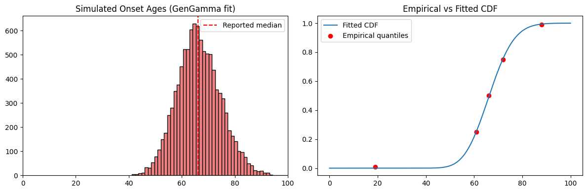
This confirms that the generalized gamma model aligns well with both the median and quartile anchors.
Adding Uncertainty: Probabilistic Sensitivity Analysis (PSA)
Why PSA?
Health economic and epidemiological models require not only point estimates but also credible intervals, especially when clinical evidence is sparse.
Parameter uncertainty in the fitted model must therefore be propagated to all downstream quantities.
The overarching goal is to generate randomly sampled, correlated parameter sets that reflect the plausible variance and covariance structure of the original fitted models for PSA.
The conceptual procedures are as follows,
- Identify the model parameters
- Build the variance–covariance matrix
- Calculate the Cholesky factor
- Generate random noise using MVN
- Apply the Cholesky factor to preserve correlations
- Compute the final random parameter draws
- Use the sampled parameters in the survival model
Building the Variance-Covariance Matrix
We approximate the Hessian numerically at the parameter optimum. Inverting the Hessian yields the variance–covariance matrix of the parameter estimates.
This matrix captures both individual parameter uncertainty and correlations among parameters.
theta_hat = np.array([a_fit, c_fit, scale_fit])
H = approx_hess(theta_hat, gengamma_objective)
vcov = np.linalg.inv(H)
| a variance/covariance | c variance/covariance | scale variance/covariance | |
|---|---|---|---|
| a | 595.13 | -17.76 | -315.06 |
| c | -17.76 | 0.55 | 9.63 |
| scale | -315.06 | 9.63 | 169.34 |
This is a 3×3 variance-covariance matrix for the 3 fitted parameters of the generalized gamma distribution.
Diagonal entries = variances of each parameter.
Example:
\[\mathrm{Var}(a) = 595.13, \quad \mathrm{Var}(c) = 0.551, \quad \mathrm{Var}(\text{scale}) = 169.34\]Off-diagonal entries = covariances between parameters.
Example:
\[\mathrm{Cov}(a, \text{scale}) = -315.06\]Multivariate Normal Sampling
Using Cholesky decomposition, we sample thousands of parameter sets from a multivariate normal distribution:
\[\theta^{(i)} \sim \text{MVN}(\hat{\theta},\, \Sigma)\]This forms the backbone of the PSA.
rng = np.random.default_rng(123)
L = np.linalg.cholesky(vcov)
Z = rng.standard_normal((5000, 3))
theta_draws = theta_hat + Z @ L.T
Even though the fitted parameters \((\mu, \log\sigma, Q)\) are point estimates, each has uncertainty, and they are correlated. For example, if log-sigma increases slightly, Q might decrease slightly to keep the model a good fit.
To reflect this, we sample parameters from a multivariate normal distribution centered at the MLE estimates with covariance equal to the Hessian-derived covariance matrix.
Here’s what the code does:
-
standard_normal((5000,3)) → generates 5,000 draws of independent noise, one for each parameter.
-
L = cholesky(vcov) → finds a matrix L such that \(LL^\top = \text{covariance}\).
This matrix converts independent noise into correlated noise with the correct variability. -
Z @ L.T → transforms the independent noise into noise that matches the covariance structure of the parameters.
-
theta_hat + … → shifts the draws so they are centered at the fitted parameters.
The resulting theta_draws are 5,000 simulated sets of generalized gamma parameters that realistically reflect estimation uncertainty. These are used to visualize uncertainty in survival curves, median survival, RMST, or other model outputs.
Estimating Age-Band Probabilities
For many models, we need to know the probability that onset occurs within:
- 0–12 years
- 12–18 years
- 18+ years
Using the CDF from each Monte Carlo draw, we compute:
\[P(a \leq \text{onset} < b) = F(b) - F(a)\]This avoids slow individual-level simulation and supports rapid PSA.
A summary table (across ~5,000 draws) includes:
- mean probability
- standard deviation
- median
- 95% uncertainty interval (2.5–97.5th percentile)
| Age Band | Mean | SD | Median | CI Lower (2.5%) | CI Upper (97.5%) |
|---|---|---|---|---|---|
| 0–12 | 2.67% | 14.00% | 0.00% | 0.00% | 44.47% |
| 12–18 | 1.95% | 9.41% | 0.00% | 0.00% | 23.81% |
| 18+ | 95.38% | 18.45% | 100.00% | 9.54% | 100.00% |
The results show:
- ~95% of onsets occur after age 18
- 0–12 and 12–18 have wide uncertainty due to very low event frequency
This output can be plugged directly into disease models.
Visualizing Uncertainty: CDF Ensembles
One of the most insightful plots overlays:
- Light gray curves: thousands of CDFs generated from sampled parameters
- A blue line: mean CDF across all Monte Carlo draws
- Red points: empirical quartile anchors
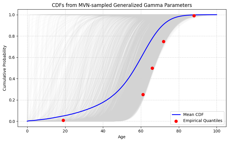
This reveals:
- Strong alignment near the median
- Greatest uncertainty in the tails
- Minimal probability mass before ~20 years
- A steep probability rise between 50–70 years
The ensemble plot illustrates not just the best-fit curve, but the range of plausible distributions given uncertainty in the literature.
Ensuring Reproducibility
Reproducibility is essential for transparent modeling, peer review, and regulatory or client submissions.
At the end of the analysis, we record:
- Python version
- OS
- NumPy, pandas, SciPy, statsmodels, matplotlib versions
Conclusion
Even when individual-level data are unavailable, we can still reconstruct a meaningful, validated age-at-onset distribution using parametric survival models.
The generalized gamma distribution offers excellent flexibility, and the combination of:
- Quantile matching
- Diagnostic validation
- Probabilistic sensitivity analysis (PSA)
This approach fits naturally into broader health economic and epidemiological frameworks, enabling:
- Estimation of onset-age probabilities
- Sensitivity and uncertainty analyses
- Population-level burden and cost projections
- Forecasting models informed by realistic evidence intervals