Reconstructing Individual Patient Data from Published Kaplan–Meier Curves in R: A Practical Guide for HEOR Analysts
Why reconstruct IPD from Kaplan–Meier curves
Many publications on rare diseases report only Kaplan–Meier (KM) curves. At the same time, HTA submissions often require individual patient data (IPD) to extrapolate survival and model long-term clinical and health economic benefits.
When IPD is unavailable, reconstructing it from published KM curves becomes an essential analytical solution.
This article introduces an R tool that enables analysts to reconstruct IPD from published KM curves using the algorithm developed by Guyot et al. (2021). This algorithm is recognized in the methodological guidance provided by the Decision Support Unit at Sheffield University, which supports the National Institute for Health and Care Excellence (NICE) Health Technology Assessment (HTA).
For full R notebook accompanying this article, see the GitHub page: https://davidzhao1015.github.io/reconstruct-ipd-km/
Required inputs before you begin
Background for published Kaplan-Meier curves
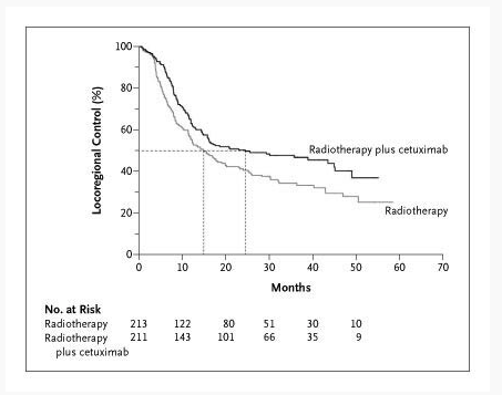
The KM curves depict time to loss of locoregional control in the treatment group, which received radiotherapy combined with cetuximab, versus the control group, which received radiotherapy alone. This data was published in an open-access New England Journal of Medicine article on skin cancer (https://www.nejm.org/doi/full/10.1056/NEJMoa053422).
According to the Cox regression analysis, the hazard ratio was 0.68 (95% CI, 0.52-0.89), as determined by the log-rank test. The dotted lines indicate the median durations of locoregional control.
Input used in example
The input data used in the official manual of the R package IPDfromKM consists of
- Time-specific event proportions for both arms
- Number of patients at risk for both arms
- Time at risk
They were digitized from KM curves and the associated life table.
Alternative input to R functions
If the life table is not reported, use the initial number of patients for analysis as a substitute for the number of patients and time at risk. At the same time, the time-specific event proportions are still warranted.
Beyond the input requirements for R functions, more flexible input types were defined by Guyot et al (2021) based on information levels,
- All information
- No number at risk
- No total events
- Neither
For a detailed introduction to the above input types, see the methodology in Guyot et al. (2021)
The R package IPDfromKM seemingly only accounts for two scenarios of information levels.
Workflow
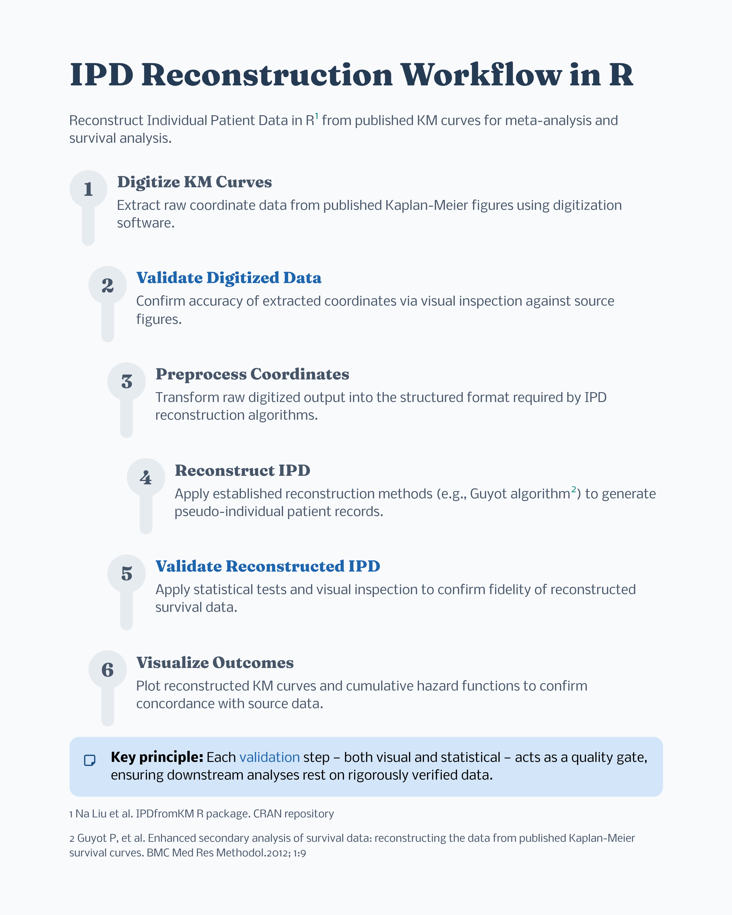
Before diving into coding nuance, the how part, I want to show a high-level workflow as a map of what parts to the audience.
The analytic workflow employed in the R package IPDfromKM is synthesized visually as follows. The two validation steps are highlighted as the quality gate, ensuring that downstream analysis relies on rigorous, verified data. The core step to reconstruct IPD is to implement the established Guyot algorithm.
Step-by-step implementation in R
Prepare data
library("IPDfromKM")

# Load example data
radio <- Radiationdata$radio
radioplus <- Radiationdata$radioplus
trisk <- Radiationdata$trisk
nrisk_radio <- Radiationdata$nrisk.radio
nrisk_radioplus <- Radiationdata$nrisk.radioplus
The object Radiation data contains four objects that represent all the input, as introduced above, needed to reconstruct survival IPD.
Validate digitized data
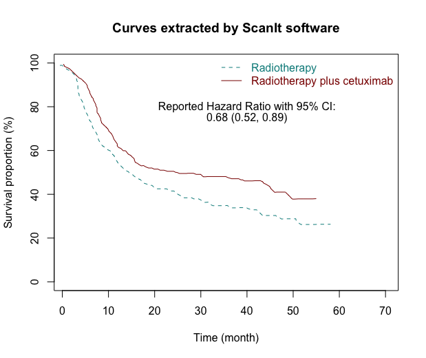
We can validate the quality of digitized input data by comparing the KM curve derived from extracted data with the published KM curve.
This example demonstrates a strong correspondence with KM shapes.
Preprocess coordinates
Convert the extracted input data into the format required for IPD reconstruction using the preprocess() function, which aligns the digitized coordinates with reported numbers at risk so that Guyot’s algorithm can correctly estimate censoring patterns.
For a complete description of arguments, see the package documentation.
If required input is available, use arguments trisk and nrisk; otherwise, use totalpts for alternative input.
# Radiotherapy treatment arm
pre_radio <- preprocess(dat = radio,
                        trisk = trisk,
                        nrisk = nrisk_radio,
                        maxy = 100)

# Radiotherapy plus cetuximab treatment arm
pre_radio_plus <- preprocess(dat = radioplus,
                             trisk = trisk,
                             nrisk = nrisk_radioplus,
                             maxy = 100)
Reconstruct IPD
Apply Guyot’s algorithm to reconstruct IPD, the core step in the procedure to estimate events and censoring based on predefined assumptions.
For example, given the number at risk, the censoring rate is assumed to distribute evenly over time intervals. If the number at risk is not available, assume there is no censoring over time intervals.
est_radio <- getIPD(prep = pre_radio, armID = 0, tot.events = NULL)

est_radio_plus <- getIPD(prep = pre_radio_plus, armID = 1, tot.events = NULL)
head(est_radio$IPD, 30)
| Patient | Time | Status | Treat |
|---|---|---|---|
| 1 | 0.00 | 1 | 0 |
| 2 | 0.00 | 1 | 0 |
| 3 | 0.26 | 1 | 0 |
| 4 | 0.78 | 1 | 0 |
| 5 | 0.78 | 1 | 0 |
| 6 | 0.78 | 1 | 0 |
| 7 | 1.03 | 0 | 0 |
| 8 | 1.29 | 1 | 0 |
| 9 | 1.81 | 1 | 0 |
| 10 | 2.07 | 1 | 0 |
| 11 | 2.33 | 0 | 0 |
| 12 | 2.59 | 1 | 0 |
| 13 | 2.59 | 1 | 0 |
| 14 | 2.85 | 1 | 0 |
| 15 | 2.85 | 1 | 0 |
| 16 | 3.11 | 1 | 0 |
| 17 | 3.11 | 1 | 0 |
| 18 | 3.11 | 1 | 0 |
| 19 | 3.11 | 1 | 0 |
| 20 | 3.24 | 0 | 0 |
| 21 | 3.37 | 1 | 0 |
| 22 | 3.37 | 1 | 0 |
| 23 | 3.37 | 1 | 0 |
| 24 | 3.37 | 1 | 0 |
| 25 | 3.37 | 1 | 0 |
| 26 | 3.38 | 1 | 0 |
| 27 | 3.38 | 1 | 0 |
| 28 | 3.38 | 1 | 0 |
| 29 | 3.38 | 1 | 0 |
| 30 | 3.38 | 1 | 0 |
The above table shows status (event or censored) and time for illustrative individual patients in the radiotherapy arm.
The codes 1 and 0 of the status column represent disease and censored, respectively.
In general, the reasons for censoring can include 1) administrative study end before event, 2) lost to follow-up, 3) withdrawal of consent, and 4) still alive at database lock. Due to limited published information, the exact reason can not be inferred.
Time represents observed follow-up duration from a defined time origin (eg., first treatment) until the patient’s last known outcome.
For example, patient 4-6 died at 0.78 months, while patient 7 was censored at 1.03 months.
Validate reconstructed IPD
The table in the first half of the summary presents a few statistics for the reconstructed IPD, including time at risk, number at risk, and estimated counts of censoring and events.
Within each interval,
- lower refers to the row index of the KM coordinates corresponding to each reported time point at which the number at risk is available;
- upper refers to the row index of the last KM coordinate before the next reported time point with available number-at-risk data.
Next, the summary presents a quantitative comparison between the reconstructed and digitized KM curves, based on root-mean-square error (RMSE), mean absolute error (MAE), and maximum absolute error. Together, these metrics indicate excellent agreement between the reconstructed and original survival curves.
As supportive evidence, the Kolmogorov–Smirnov (KS) test showed no statistically significant difference between the distributions of the reconstructed and digitized survival probabilities (D = 0.076, p = 0.795), indicating that the reconstructed KM curve provides an excellent approximation of the published survival curve.
> summary(est_radio)

The function read in  144 points from the K-M curve and 6 numbers of patients at risk.
Thus the read-in points are divided into  6 time intervals.

 interval lower upper trisk nrisk nrisk.hat censor.hat event.hat
        1     1    42     0   213       213          8        83
        2    43    66    10   122       122         10        32
        3    67    88    20    80        80         19        10
        4    89   109    30    51        51         16         5
        5   110   129    40    30        30         17         3
        6   130   144    50    10        10          9         1

The root-mean-square error between estimated and read-in survival probabilities is 0.004.
The mean absolute error between estimated and read-in survival probabilities is 0.003.
The maximum absolute error between estimated and read-in survival probabilities is 0.013.

The Kolmogorov-Smirnov test:
Test statistics D= 0.07639       p-value= 0.7948
Null hypothesis: distributions of the read-in and estimated survival probabilities are the same.
In HTA work, reconstruction quality determines the credibility of downstream survival extrapolation. It is advisable to review RMSE, MAE, KS statistics, and graphical diagnostics together before considering the reconstructed IPD sufficiently reliable for modeling.
Visual inspection
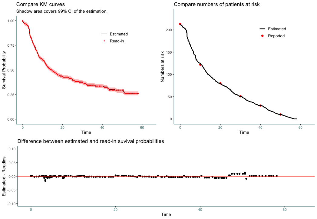
The IPDfromKM package provides graphical diagnostics to assess how well the reconstructed IPD reproduces the published KM curves and the digitized source data.
The three subplots provide a comprehensive evaluation of the quality and validity of the reconstructed IPD:
- Top left: The digitized KM data points closely follow the reconstructed survival curve and generally fall within the estimated 95% confidence interval, indicating good agreement.
- Top right: The numbers at risk derived from the reconstructed IPD closely match the reported numbers at risk throughout follow-up, demonstrating that the reconstruction preserves the underlying risk set.
- Bottom: The differences between the reconstructed and digitized survival probabilities are small across time, indicating that the reconstructed IPD accurately reproduces the published KM curve.
plot(est_radio)
Visualize outcomes
Once the reconstructed IPD has been validated, it can be used to answer several clinically and statistically important questions that are often not directly reported in the original publication.
An HTA submission requires extrapolating overall survival beyond a clinical trial. Only published KM curves are available. Reconstructed IPD allows fitting alternative parametric models for extrapolation.
All the above insights can be generated by calling a single function, survreport().
surv2 <-survreport(ipd1 = est_radio$IPD,
                   ipd2 = est_radio_plus$IPD,
                   arms = 2,
                   interval = 8,
                   s = c(0.75, 0.5, 0.25),
                   showplots = TRUE)
Understanding and validating the outputs
Quantitative outcomes
- $survtime: Median survival time. Estimate when 50% of patients have experienced the event (e.g., death or disease progression) in the control and treatment arms.
- $survprob: Uncertainty around survival estimates. Quantify the uncertainty surrounding point estimates using confidence intervals and statistical inference.
> surv2$arm1
$survtime
                 time 0.95LCI 0.95UCI
survprob = 0.75  5.73    4.68    7.55
survprob = 0.5  14.80   11.70   23.10
survprob = 0.25    NA      NA      NA

$survprob
            Surv     SE 0.95LCI 0.95UCI
time = 8  0.6507 0.0330  0.5890  0.7187
time = 16 0.4808 0.0350  0.4168  0.5545
time = 24 0.4151 0.0350  0.3519  0.4897
time = 32 0.3611 0.0353  0.2981  0.4374
time = 40 0.3356 0.0358  0.2723  0.4136
time = 48 0.2964 0.0382  0.2303  0.3815
time = 56 0.2635 0.0460  0.1871  0.3710
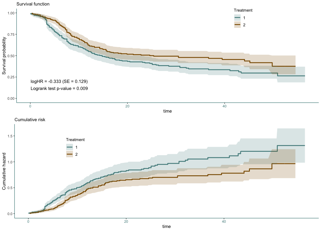
Reconstructed KM curves
- Top: Treatment effect. Estimate the hazard ratio (HR) between arms and assess whether the difference is statistically significant.
- Treatment arm (Treatment 2, brown) has consistently higher survival probabilities than the control arm (Treatment 1, blue).
- Patients receiving the treatment have about a 28% lower instantaneous risk of experiencing the event than patients receiving the control.
- The difference between the survival curves is statistically significant at the 5% level.
- Bottom: Proportional hazards assumption. Evaluate whether the proportional hazards assumption is reasonable by inspecting the log-cumulative hazard plot over time.
- Patients in the control arm (Treatment 1) experience events at a higher rate over time than patients in the treatment arm (Treatment 2), after the initial period (5-10 months).
- Both arms have steepest increases early and flatten over time.
- Two curves are roughly parallel after the initial period, indicating the proportional hazard assumption might hold.
- Confidence intervals become wider over time, as expected, because patients at risk are fewer, censored patients accumulate, and precision decreases.
Recommended practice for high reconstruction accuracy
Guyot et al (2012) emphasize a few significant practices for reconstruction accuracy, particularly for hazard ratios. Below, I briefly summarize those points as follows to help the audience achieve better results using the above methodology.
- Essential data inputs: The “full-information” case leads to the most reliable results for hazard ratios, which consists of digitized KM curve coordinates, number at risk, and total event numbers. Without number at risk and total number of events, hazard ratios may be “frankly unusable”.
- Quality of the original image: The published KM curve should not be blurry, and the numerical axis scales must be clear.
- Careful digitization: Every “step” visible in the KM curve should be captured by a data point to ensure sufficient data, with careful care.
- Data consistency: Extracted coordinates must be consistent. Any abnormalities due to human error or poor publication quality must be corrected before running the algorithm.
- Inclusion of risk time points: The specific times when the numbers at risk are reported must be included in the initial digitized data points.
Limitations, assumptions and uncertainty
Understanding the limitations and key assumptions of the algorithm is essential to avoid misleading inputs and to inform uncertainty analysis for health economics modeling.
- The accuracy of reconstructed results, particularly hazard ratios, depends on the quality and completeness of the source data. Either missing numbers at risk, absent total events, or unclear images or axis scales can all reduce the reliability of extracted information and subsequent analyses.
- Human error during digitization and pre-processing can introduce inaccuracies in the reconstructed data. Attention to detail in these steps is essential to minimize such risks and maintain data integrity.
- Unlike true individual patient data (IPD), reconstructed data from published survival curves reflect only pooled summary information. This limitation means subgroup-specific curves cannot be generated, and joint effects of treatments and covariates cannot be modeled, increasing the risk of aggregation bias.
- The algorithm must also make assumptions about censoring patterns, often defaulting to a constant rate within intervals. If neither numbers at risk nor total events are provided, the algorithm assumes no censoring, which can underestimate the uncertainty of hazard ratio estimates.
- If the original data violate the proportional hazards assumption, the accuracy of reconstructed hazard ratios may be further compromised.
Utilizing uncertainty analysis in health economic modeling, such as probabilistic sensitivity analysis and scenario analysis, can help address the aforementioned assumptions.
Where reconstructed IPD fits into HEOR modeling
Reconstructing IPD is essential for HEOR modeling because it enables the generation of robust evidence from trial data. It enables precise KM estimation, Cox regression, and parametric survival modeling to clearly demonstrate clinical value.
With reconstructed IPD, analysts can project long-term clinical value benefits in health economic models by extrapolating survival beyond observed follow-up, directly supporting value communication.
References
- Guyot, P., Ades, A. E., Ouwens, M. J. N. M., & Welton, N. J. (2012). Enhanced secondary analysis of survival data: Reconstructing the data from published Kaplan–Meier survival curves. BMC Medical Research Methodology, 12, 9. https://doi.org/10.1186/1471-2288-12-9
- Latimer, N. R. (2013). NICE Decision Support Unit Technical Support Document 14: Survival analysis for economic evaluations alongside clinical trials – Extrapolation with patient-level data. National Institute for Health and Care Excellence (NICE) Decision Support Unit.
- Liu, N., Zhou, Y., & Lee, J. J. (2025). IPDfromKM: Reconstruct individual patient data from Kaplan–Meier survival curves (R package, Version 0.5.6). Comprehensive R Archive Network. https://cran.r-project.org/package=IPDfromKM
- Liu, N., Zhou, Y., & Lee, J. J. (2025). IPDfromKM Reference Manual. Comprehensive R Archive Network. https://cran.r-project.org/web/packages/IPDfromKM/refman/IPDfromKM.html
- Bonner, J. A., Harari, P. M., Giralt, J., Azarnia, N., Shin, D. M., Cohen, R. B., Jones, C. U., Sur, R., Raben, D., Jassem, J., Ove, R., Kies, M. S., Baselga, J., Youssoufian, H., Amellal, N., Rowinsky, E. K., & Ang, K. K. (2006). Radiotherapy plus cetuximab for squamous-cell carcinoma of the head and neck. New England Journal of Medicine, 354(6), 567–578. https://doi.org/10.1056/NEJMoa053422