How to Model Correlated Parameter Uncertainty in Excel Using Cholesky Decomposition
Background
In probabilistic sensitivity analysis (PSA), widely used in health economic and epidemiological modeling, it is considered good practice to incorporate uncertainty not only in input parameters but also in fitted statistical model parameters. For instance, age at disease onset distributions or transition survival functions between health states are often estimated using parametric models.
However, these fitted parameters behave differently from typical PSA inputs such as costs, utilities, or prevalence estimates. Parameters derived from statistical models are usually correlated with one another, meaning they cannot be sampled independently without potentially distorting the model structure.
To address this, uncertainty must be introduced in a way that preserves the correlation structure while still allowing stochastic sampling during simulation.
In this post, I walk through a practical modeling architecture designed to handle this challenge. The approach has been applied in real-world modeling projects, and the article explains both the key mathematical components and the statistical intuition behind them. The goal is to help analysts understand how to implement correlated parameter uncertainty in PSA and adapt the template to their own models in Excel.
For readers who are comfortable with Python, a companion post is also available that demonstrates how to implement uncertainty analysis for fitted survival model parameters within the Python ecosystem.
Practical explanation of Cholesky decomposition and multivariate normal distribution
Intuitively, the idea is simple. When we generate random numbers independently, they have no relationship with each other. However, parameters estimated from statistical models often move together, if one parameter increases, another may tend to increase or decrease as well. This relationship is captured in the covariance matrix.
Cholesky decomposition converts this covariance matrix into a transformation matrix that can reshape independent random draws into correlated ones. In practice, we first generate a vector of independent standard normal random variables, and then multiply this vector by the Cholesky matrix. The transformation introduces the appropriate covariance structure, ensuring that the simulated parameters follow the same correlation pattern observed in the original model estimates.
As a result, each probabilistic sensitivity analysis iteration reflects plausible combinations of parameters, rather than unrealistic values that could arise if parameters were sampled independently.
In practical HEOR or epidemiology models, the covariance matrix is extracted from the fitted survival or regression model and used to generate correlated parameter draws for PSA. The diagram representation of the procedure is as below.
Model fitting → covariance matrix → Cholesky → parameter sampling → simulation → outcomes
Step-by-step guide
Use Case
A common application of this approach is incorporating fitted parameters from a lognormal model into PSA. Lognormal models are frequently used to represent time-to-event outcomes, such as age at disease onset or survival distributions.
The lognormal model contains two parameters, μ (mu) and σ (sigma), which represent the mean and standard deviation of the underlying normal distribution on the log scale. These parameters are typically estimated simultaneously during model fitting and are therefore correlated.
In PSA simulations, the model requires randomly sampled parameter values for each iteration. To ensure realistic uncertainty propagation, the sampled values of μ and σ should preserve their estimated correlation, rather than being drawn independently.
The approach described in this post demonstrates how correlated samples of these parameters can be generated and incorporated into PSA simulations.
Worksheet Setup
In this section, we walk through the worksheet architecture used to implement probabilistic sensitivity analysis (PSA). The structure includes:
- a Helper sheet used to compute the Cholesky matrix (factors) required for correlated parameter sampling, and
- a Parameter sheet that stores model inputs and generates probabilistic parameter values used in PSA simulations.
Helper Sheet
The Helper sheet is used to calculate the Cholesky matrix (or Cholesky factors) based on the variance–covariance matrix obtained from the statistical model. These factors are then used to transform independent random draws into correlated parameter samples for PSA simulation.
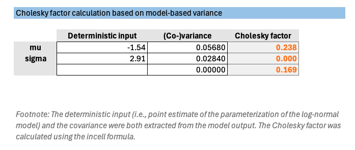
Co-variance values are extracted from the fitted model and describe the correlation between the estimated parameters, typically obtained from statistical modeling software such as R or Python.
The calculation formulas are shown in the Cholesky factor columns for reference.
1) Start from covariance matrix
Suppose you have:
\[\Sigma = \begin{bmatrix} \operatorname{Var}(\mu) & \operatorname{Cov}(\mu,\sigma) \\ \operatorname{Cov}(\mu,\sigma) & \operatorname{Var}(\sigma) \end{bmatrix}\]For example, from your model output:
\[\Sigma = \begin{bmatrix} 0.258491 & 0.000002 \\ 0.000002 & 0.129243 \end{bmatrix}\]Therefore:
- \[Var(mu) = 0.258491\]
- \[Var(sigma) = 0.129243\]
- \[Cov(mu,sigma) = 0.000002\]
2) Cholesky factor
For a 2×2 covariance matrix, the lower triangular Cholesky matrix is:
\[L = \begin{bmatrix} L_{11} & 0 \\ L_{21} & L_{22} \end{bmatrix}\]where:
\[L_{11} = \sqrt{\operatorname{Var}(\mu)}\] \[L_{21} = \frac{\operatorname{Cov}(\mu,\sigma)}{L_{11}}\] \[L_{22} = \sqrt{\operatorname{Var}(\sigma)-L_{21}^2}\]3) Excel formulas for Cholesky cells
Assume:
- B2 = variance of mu
- B3 = covariance(mu, sigma)
- B4 = variance of sigma
Then the Cholesky elements can be calculated as:
L11
=SQRT(B2)
L21
=B3/SQRT(B2)
L22
=SQRT(B4-E3^2)
If E3 holds L21
As a validation checkpoint, the Excel formula–based Cholesky factors were compared with values programmatically calculated using the lifelines package in Python, and the results showed close agreement.
Parameter Sheet
The screenshot below illustrates the structure of the Parameter sheet. Key columns include deterministic values, probabilistic values, standard deviations, and covariance terms.
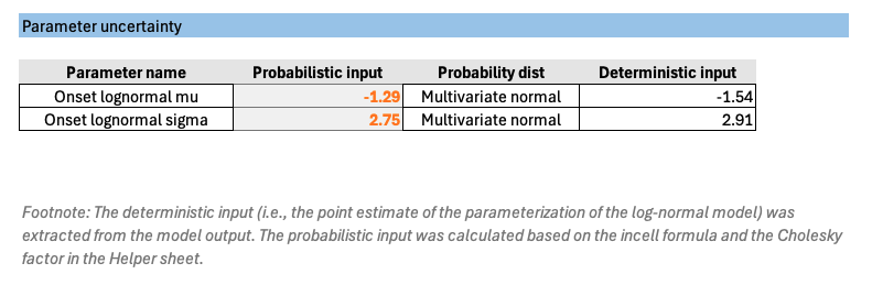
- Deterministic input represent the point estimates of the fitted model parameters, such as μ and σ from the lognormal model.
- Probabilistic value column contains formulas that generate random samples of model parameters for each PSA iteration. These formulas incorporate the correlation structure between parameters.
Generating correlated parameter draws
For a standard 2-parameter lower-triangular Cholesky matrix as above, the simulated parameter values are generated as:
\[\mu^* = \mu + L_{11}Z_1\] \[\sigma^* = \sigma + L_{21}Z_1 + L_{22}Z_2\]where:
- L11 represents the Cholesky factor associated with μ
- L21 and L22 represent the Cholesky factors associated with σ
The random variables are:
Z1 = NORM.S.INV(RAND())
Z2 = NORM.S.INV(RAND())
where Z1 and Z2 are independent standard normal random variables.
Excel formula
Assume:
Helper!G8 = L11
Helper!G9 = L21
Helper!G10 = L22
Parameter!G6 = mu (point estimate)
Parameter!G7 = sigma (point estimate)
=NORM.S.INV(RAND())*Helper!G8 + Parameter!G6
=NORM.S.INV(RAND())*Helper!G9 + NORM.S.INV(RAND())*Helper!G10 + Parameter!G7
These random draws are then transformed using the Cholesky factors, producing correlated samples of μ and σ that reflect the uncertainty and covariance structure estimated from the statistical model.
Optional: Check Sheet
To validate the robustness of the procedure described above, a Check sheet is included in the template. This sheet provides a graphical illustration of the simulated distribution curves, for example the cumulative proportion of patients who have not yet developed symptoms over time.
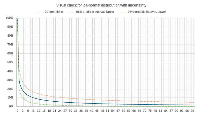
The chart also displays the upper and lower bounds of the 95% credible interval, derived from 100 PSA iterations using randomly sampled curve parameters.
This visual diagnostic helps verify that the sampling architecture and parameterization behave as expected, ensuring that the simulated curves reflect both the central estimate and the uncertainty captured by the fitted model parameters. Such graphical checks provide a practical way to confirm that the PSA implementation is functioning correctly before applying the model in downstream analyses.
Re-usable Excel template
The reusable Excel template is available in the GitHub repository. Embedded guiding notes within the workbook help users navigate the template and identify where to enter the required input values.
The formula-based calculations in the Excel template have been cross-validated against Python-based results to ensure consistency and accuracy.
Feedback is always welcome. Please feel free to leave comments or suggestions to help improve the template for future users.