How to Reconstruct Partitioned Survival Curves from Hazard Ratios

Introduction

How can analysts translate a hazard ratio into a full partitioned survival curve suitable for economic modeling?

Imagine a gene therapy sponsor is preparing a cost-effectiveness model for a rare neuromuscular disease.

The standard-of-care model is already available, but evidence for a competing therapy consists only of a published hazard ratio for disease progression.

The sponsor must estimate how patients would distribute across disease stages over a lifetime horizon in order to quantify:

quality adjusted life year (QALY)
costs
incremental value (ICER)

The article shows how to establish an analytic framework and simulate comparative survival distributions using base-case and trial-informed hazard ratios.

This article introduces partitioned survival models. If you want more on survival modeling approaches, please refer to our previous article for additional details.

Fundamental statistical concepts

The analytical workflow centers on three key statistical concepts: the partitioned survival model (PSM), the Markov transition model, and hazard calculation.

A main input is the PSM’s results. The estimated transition probability matrix serves as a proxy for the Markov model’s results and directly connects to the hazard ratio, another input. By understanding how hazard and transition probability are linked, one can rebuild the Markov transition matrix using hazard ratios.

Partitioned survival model

The Partitioned Survival Model (PSM) is often used in my collaborative work to track rare diseases over time.

In modeling, a cohort is a group of patients tracked over time. PSM splits the cohort into distinct health states (i.e., disease stages). The proportion of patients at each stage is estimated using parametric survival models, mathematical tools for analyzing time-to-event data.

A key assumption for PSM is that patients only move to worse disease stages over time and cannot improve. This assumption is very important when using PSM.

PSM can be applied to cancer trial data and extended with mathematical models, such as Weibull and log-normal, to estimate lifetime survival times. This makes PSM a useful approach for estimating long-term health effects from trial data. PSM always works with groups of patients, not individuals.

Markov (transition) model

The Markov transition model shows how patients move between different health states based on the probabilities of transitions between them.

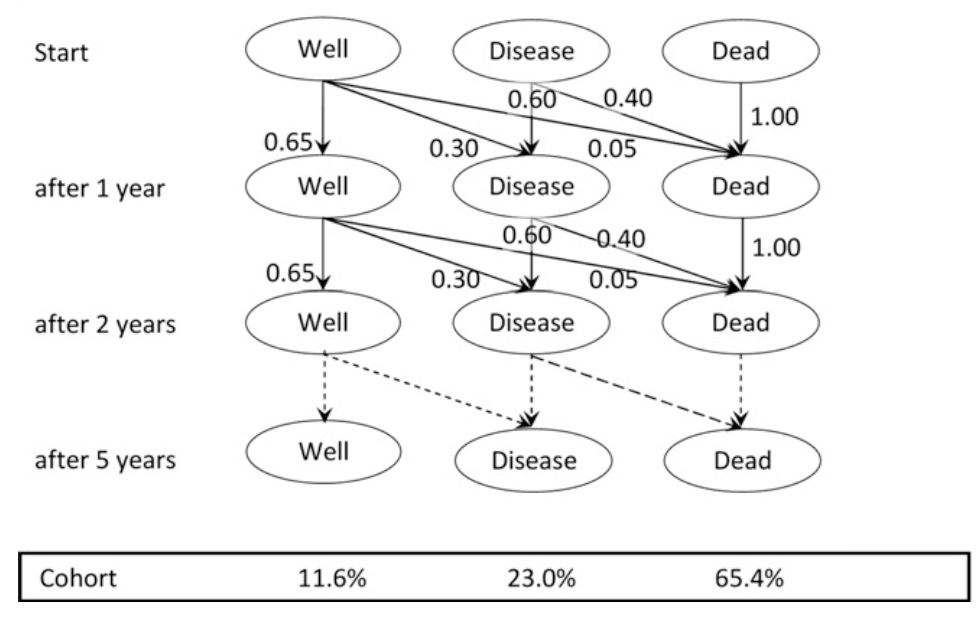
Figure 1. Bubble diagram illustrating the state-transition model, derived from the ISPOR best practice paper. The entire cohort is distributed across states, well, disease and dead after each cycle.

The Markov transition model is based on the assumption that the probability of moving between states depends only on the current state and time, not on what happened earlier. It allows for staying in the same state or moving between many health states.

Markov models are often used to estimate costs and health benefits for each period, such as monthly or annually.

A Markov model is usually used for groups of patients, but it can also be used for one patient at a time, sometimes called micro-simulation.

Table 1. Comparison between PSM and the Markov model

Question	PSM	Markov Model
What proportion of patients are in each disease state over time?	Primary focus	Derived from transitions
How do patients move between disease states?	Not explicitly modeled	Primary focus
Can patients improve or move between multiple states?	Usually no	Yes
Can the model simulate an individual patient?	No	Yes (microsimulation)

The above insights are attributed to Hannah Gillies and Mirko von Hein, who offer high-quality video tutorials on the topics. For more on PSA and Markov models, I recommend that the audience check out the resources cited in the Reference section.

Relationship between internal hazard and transition probability

Hazard h is not a probability. Hazard represents the continuous risk intensity acting on individuals who have not yet experienced the event.

The exponential survival model assumes that the hazard is constant over the time interval.

$p=1-e^{-h}$

where,

p = probability of the event during the interval
h = constant hazard during the interval

Thus,

$h=-\ln(1-p)$

Understanding the mathematical conversion between event probability and hazard is central to inferring a target probability distribution from the demanded hazard ratio.

The analytical workflow is shown below,

Obtain the annual transition probability from the literature.
Convert to hazard:

$h=-\ln(1-p)$

Apply hazard ratios:

$h_{new}=HR\times h_{base}$

Convert back to probability:

$p_{new}=1-e^{-h_{new}}$

This probability → hazard → apply HR → probability workflow is standard when combining evidence from different sources.

Step-by-step walkthrough for the Excel template

Use case context

The calculation structure is organized into a four-stage progression of a rare disease.

The health states are labeled generically as HS1, HS2, HS3, and HS4, with an additional state for death. The generic health states can be mapped to the following clinical example.

Generic state	Clinical example
HS1	Ambulatory
HS2	Early functional decline
HS3	Non-ambulatory
HS4	Severe disability
Death	Mortality

Figure 2. Conceptual disease progression from HS1 to HS4 to death. The arrows indicate the direction of disease progression, which is unidirectional and irreversible.

The quantifications of base partitioned curves represent the modeled output of partitioned survival models (PSM) for the rare disease.

As mentioned in the section on fundamental statistical concepts, we assume patients can only transition to a worse health state, not in the reverse direction, in line with the partitioned survival model’s principle.

The transition-specific hazard ratios are based on dummy data.

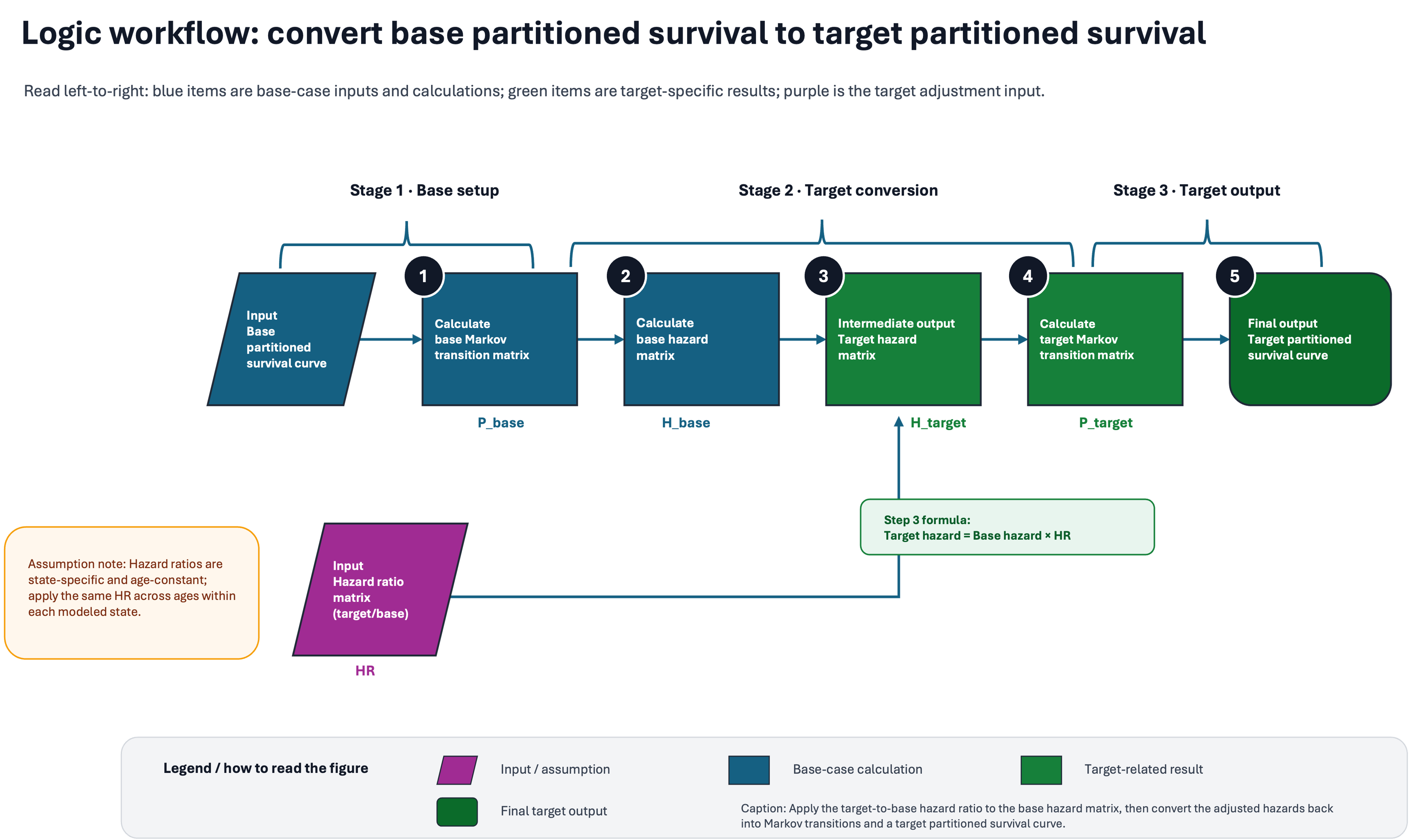
Overview

The analytic workflow illustrates five steps for inferring target-partitioned survival from the base survival. The entire procedure consists of three stages: base step, target conversion, and target output.

The legend box describes how to interpret the diagram. In brief, shapes represent input, intermediate results, and final output, and color coding represents types of data, base- or target-related data, or hazard ratios.

As highlighted in the light yellow box, the key assumption is that hazard ratios (HRs) are state-specific and age-constant, applying the same HR across ages within each modeled state.

In the subsequent sections, I will walk through each step of the logic workflow.

Figure 3. Logic workflow to convert base partitioned survival to target partitioned survival

Input

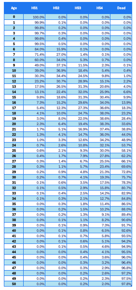
Two pieces of input data are required: a base partitioned survival curve (Table 1) and transition-specific hazard ratios (Table 2).

As mentioned above, the values in Table 1 are derived from the model’s output for a rare disease, while the values in Table 2 are dummy data.

In Table 1, the first column shows the cohort ages, while the remaining columns show the health state (HS) of surviving patients (HS1-4) and the death status of deceased patients.

In the use case, the lifetime horizon is 50 years. The sum of the proportions of patients across the four health states, plus the proportion of patients who are dead, equals 100%.

Table 1. Partitioned survival curve of the base case

In Table 2, the left column shows hazard ratio values, and the right column shows the corresponding transition steps. The detailed quantification is dummy for the use case.

In general, HR of 1 means no difference in two hazards between base and target; while HR less than 1 means the target’s hazard is lower than that of the base. For more details on hazards and hazard ratios, recommend that the audience read another blog article.

In this use case, the target hazard is 20% relative to the base during the transition from HS2 to HS3. In contrast, the hazard remains unchanged for other transition steps between target and base scenarios.

Table 2. Transition-specific hazard ratios

HR	Transition
1	HS1-HS2
0.2	HS2-HS3
1	HS3-HS4
1	HS4-Death

A hazard ratio of 0.20 for HS2→HS3 implies that patients progress much more slowly from early functional decline to loss of ambulation.

If the hazard ratio for HS2→HS3 is 0.20, the expected implications:

More patients remain in HS2.
Fewer patients reach HS3 and HS4.
QALYs increase
Medical costs may decrease.
ICER may improve

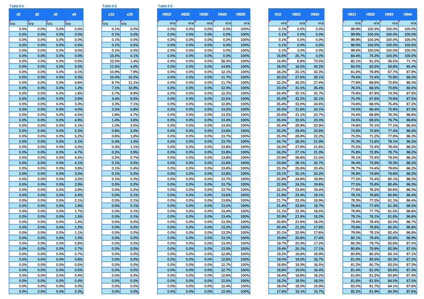
Calculation base Markov matrix (Step 1 in workflow chart)

The first step in the calculation is to reconstruct a base Markov matrix (Table 3-3. Transition probability). Although the Markov matrix is not from standard Markov modeling, it is similarly characterized by matrix structure and probability.

Breakdown of the set of intermediate results is shown below,

Table 3-1 Death proportion, health state specific. Intermediate result of the calculated death proportions from each individual HS of a given age. Assume that only HS4 patients will progress to death, while the other three HS will not.
Table 3-2 Helper columns. A helper table that includes calculated patient proportions transitions from HS1 to HS2 and from HS2 to HS3.
Table 3-3 Transition probability. A set of tables that includes estimated probability transitions from the corresponding two HS indicated in the column headers at a given age.

The calculation formula is detailed in the in-cell formula in the template spreadsheets. Understanding patient flows, progress toward worse health states, or staying at the same health states under the PSM assumption can help interpret the calculation methods.

Table 3. A set of intermediate results for the calculation of the base Markov matrix

Target conversion (Step 2-3 in workflow chart)

After reconstructing the transitional probability matrix, calculate the base hazard. Next, infer the target hazard using the given input hazard ratios.

Table 4. A set of intermediate results for target conversion

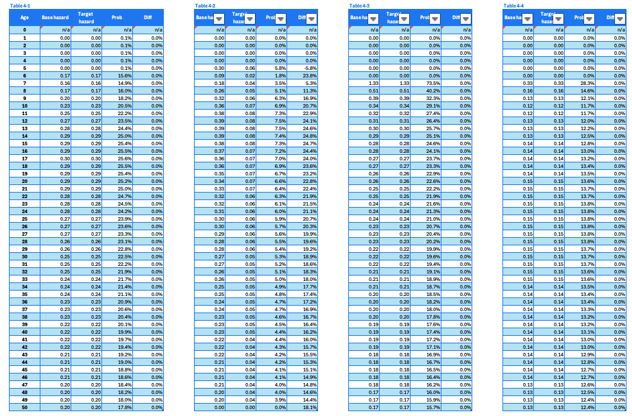
Review the four sub-tables corresponding to the transitions HS1-HS2, HS2-HS3, HS3-HS4, and HS4-death, organized from left to right.

Each sub-table has the same structure. For example, Table 2-5 can be used for explanation. The columns are:

Age: 0 to 50 years. This column shows the follow-up period or extrapolation horizon for both cohorts.
Base hazard: Hazard calculated for the base cohort using transitional probabilities.
Target hazard: Hazard inferred for the target cohort, based on the base hazard and hazard ratio.
Prob: Calculated transitional probability based on target hazard
Diff: Difference between base transitional probability and target transitional probability.

Calculate the target Markov matrix (Step 4 in workflow chart)

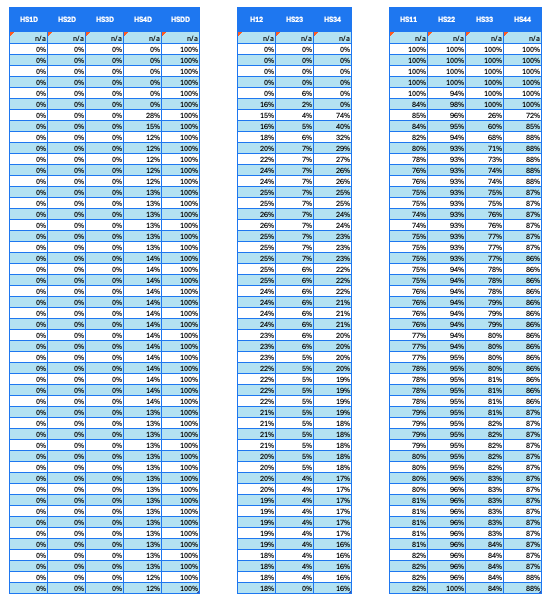
With prior calculations complete, reconstruct a Markov matrix for the target cohort.

Each cell shows a transitional probability specific to the age (row). It also corresponds to the transition between two health states (as shown in the column).

The column headers indicate particular transitions. For example, HS1D represents the shift from HS1 to death. HS12 represents the shift from HS1 to HS2.

In this use case, only the HS2-to-HS3 transition has a different probability than in the base cohort. All other transitions have the same transition probability as the base cohort.

Table 5. Consolidation of derived probabilities specific to HS transitions, as indicated in the column headers.

Target partitioned survival curve (Step 5 in workflow chart)

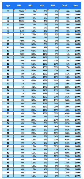
Finally, convert the Markov transition matrix to cumulative proportions of patients at individual health states.

Table 6 shows age-specific proportions of patients in the target cohort, with four health states and death. The Sum column is for validation purposes.

Table 6. Target partitioned curve reconstructed based on base-case curves and transitional hazard ratio.

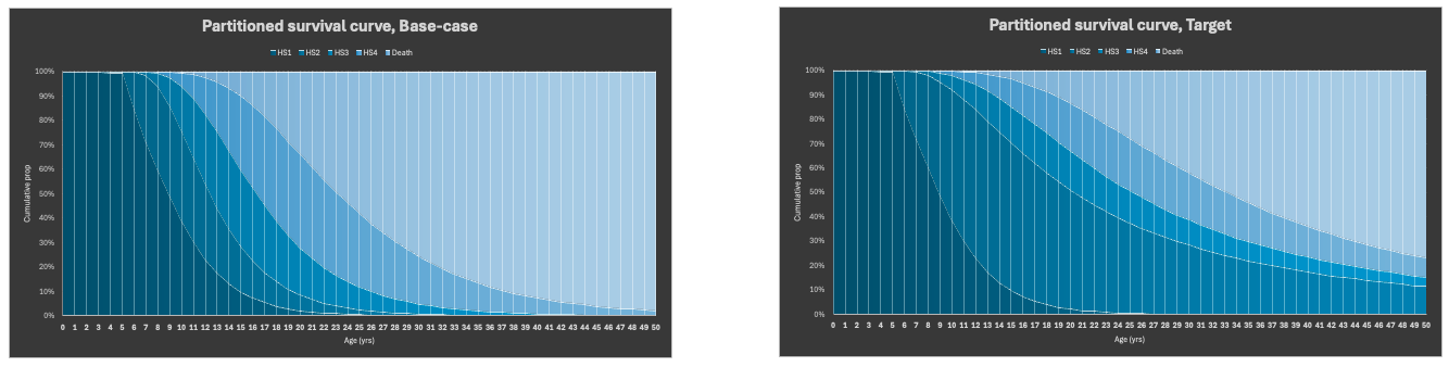
Graphic output

To assess whether the above multi-step procedure is appropriate, first visualize the base and target partitioned survival curves using area charts. This initial visualization facilitates the subsequent interpretation.

From 6 to 50 years, a relatively greater proportion of patients remain in the HS2 stage and transition more slowly to worse health states (HS3, HS4, and death), as visually confirmed by the charts, supported by mathematical calculations, and corroborated by clinical interpretation.

Figure 4. Comparison of base and target partitioned survival curves

Validation checks

We can validate the reconstructed partitioned survival curves from the following aspects,

proportions sum to 100%
State transitions are monotonic.
Survival curves are clinically plausible.

Key assumptions

Two key assumptions are inherent in the analytic framework,

Constant transitional probability during an age interval
Constant hazard ratio during an age interval

Impact of assumptions in decision-making

The treatment effect can vary by age or follow-up duration. Real-world hazard ratios may differ from assumed constants, often based on trial data with limited follow-up.

Analysts are advised to interpret model outputs with these inherent uncertainties in mind.

How to address the limitation

To address this, analysts can apply sensitivity analysis to factors such as

Comparing different hazard ratios.
Incorporate age-specific hazard ratios based on the best available evidence.

Future directions

Expand the input structure to include age-specific hazard ratios, rather than relying solely on transitions. With this expansion, we can reduce uncertainty by using consistent hazard ratios across ages and avoid overly optimistic modeling results.
Integrate general population morality adjustment.
Enhance the template’s flexibility to accommodate arbitrary numbers of health states beyond the fixed four in the use case.

References

Hannah Gillies. What is a partitioned survival model? [Video]
Hannah Gillies. What is a Markov model? - Health economics model structures [Video]
Mirko von Hein. Cost-Effectiveness Models Explained: Which One is Right for Your Analysis [Video]
Siebert, U., Alagoz, O., Bayoumi, A. M., Jahn, B., Owens, D. K., Cohen, D. J., Kuntz, K. M., & ISPOR-SMDM Modeling Good Research Practices Task Force (2012). State-transition modeling: a report of the ISPOR-SMDM Modeling Good Research Practices Task Force–3. Value in health : the journal of the International Society for Pharmacoeconomics and Outcomes Research, 15(6), 812–820. https://doi.org/10.1016/j.jval.2012.06.014