Survival Model Selection and Validation for HEOR in R
Introduction
In health economic evaluations such as cost-effectiveness analyses, long-term health benefits over a lifetime horizon are essential, but randomized controlled trials (RCTs) typically have short follow-up periods.
In accordance with health technology assessment (HTA) guidelines, survival data should be extrapolated in a statistically sound and clinically reasonable way to predict life expectancy for both the new treatment and the standard of care.
The tutorial article, translated from an R notebook, offers a reusable framework for HTA when fitting survival models and evaluating selected models in economic evaluation.
Comprehensive workflow and R tools
NICE-recommended survival extrapolation workflow
The NICE TSD14 suggests a well-structured four-step method so survival extrapolations are both statistically sound and clinically credible.
Each step follows the previous one, guiding the analyst from exploratory data inspection to a final model selection that can be properly justified and withstand examination in a health technology appraisal.
Step 1 — Assess model assumptions & hazard structure
Begin with graphical and statistical tools to identify plausible survival and hazard shapes before selecting a model. Use this check to set up the candidate models that follow.
Step 2 — Fit candidate models
Fit the full standard parametric family (Exponential, Weibull, Gompertz, Log-normal, Log-logistic, Generalized Gamma) and flexible alternatives (e.g., piecewise or flexible modeling) when justified.
Step 3 — Evaluate statistical fit & graphical diagnostics
Compare fitted curves against the Kaplan-Meier estimate and AIC. Visually inspect Q-Q and Cox-Snell residual plots to detect systematic departures. Use these results to narrow the candidate set before external review.
Step 4 — Evaluate external validity & decision uncertainty
Assess whether extrapolated curves are clinically plausible, consistent with external evidence, and robust to alternative model choices. Use this check after the internal fit assessment.
Step 5 — Model selection and structural uncertainty
Select the model by weighing statistical fit, graphical diagnostics, clinical plausibility, and external validation. Then compare plausible alternatives to assess structural uncertainty and its impact on decision-making. This completes the selection process and leads into scenario analysis.
R packages
Three specialized R packages were used to implement the workflow:
- survival: Fit Kaplan-Meier curves and create visualizations (e.g., cumulative hazard plots)
- flexsurv: Fit parametric and flexible survival models, perform residual diagnostics, and create visualizations
- GofCens: Assess goodness of fit and create visualizations
Input data
The input data, censored time-to-event data (locoregional control), were digitized from an RCT by Bonner et al., 2006, investigating the effect of cetuximab treatment on patients with head and neck cancer.
Inspect the first rows of the combined dataset. The columns are defined as follows:
- time: Follow-up time in months.
- status: 1 indicates an event; 0 indicates censoring.
- treat: 1 indicates treatment; 0 indicates control.
| ID | time | status | treat |
|---|---|---|---|
| 1 | 0.00274 | 1 | 0 |
| 2 | 0.00274 | 1 | 0 |
| 3 | 0.26100 | 1 | 0 |
| 4 | 0.77900 | 1 | 0 |
| 5 | 0.77900 | 1 | 0 |
| 6 | 0.77900 | 1 | 0 |
| 7 | 1.03450 | 0 | 0 |
| 8 | 1.29000 | 1 | 0 |
| 9 | 1.81000 | 1 | 0 |
| 10 | 2.07000 | 1 | 0 |
Step 1 - Assess model assumptions & hazard structure
Start with graphical and statistical tools to determine plausible survival and hazard shapes. Use that assessment to guide the next modeling steps.
Step 1.1 Log cumulative hazard plot
A (log) cumulative hazard plot is recommended to answer key questions:
- What hazard structure is supported?
- Are proportional hazards (PH) reasonable?
To assess whether hazards are constant over time (e.g., exponential distribution), plot cumulative hazard versus time. To evaluate monotonic hazard changes (e.g., Weibull and Gompertz distributions), plot the logarithm of cumulative hazard against the logarithm of time.
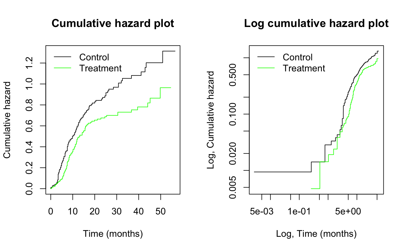
The cumulative hazard curves (left) change slope around 10–20 months, suggesting the hazard may vary over follow-up. A constant-hazard exponential model therefore appears questionable over the full period. Piecewise or more flexible models may be worth considering.
On the log-cumulative-hazard scale (right), approximate linearity over a sustained interval supports further consideration of Weibull-type models. Examine early and later departures from linearity before concluding one distribution is suitable. Evaluate Gompertz and other families using appropriate distribution-specific diagnostics.
The treatment-arm curves (right) appear approximately parallel over parts of follow-up, but early instability and possible time-varying separation mean PH is not clearly established. Consider PH provisional and assess it alongside residual-based tests and clinical expertise. If PH is not supported, consider arm-specific or time-varying approaches.
Step 2. Fit common parametric survival models to both arms
Fit the same candidate distribution type to both arms, allowing arm-specific scale and, when appropriate, shape parameters. Use a treatment-covariate PH parameterization only if PH is supported. If you select different distribution families for the two arms, explain why with strong statistical, biological, and clinical evidence. This keeps the model-building step aligned with the earlier hazard assessment.
Step 3. Evaluate statistical fit & graphical diagnostics
Step 3.1 Evaluate the AIC of fitted models
Evaluate the relative fit of models fitted to the same observed data, accounting for model complexity, using the Akaike information criterion (AIC).
AIC does not establish absolute adequacy, robustness, or credibility of the extrapolated tail; those questions require graphical diagnostics, assessment of censoring, clinical plausibility, and external validation. Perform those checks before finalizing a model.
| Distribution | AIC |
|---|---|
| gompertz | 2173.631 |
| llogis | 2179.306 |
| gengamma | 2191.250 |
| lognormal | 2198.150 |
| weibull | 2204.574 |
| exponential | 2215.113 |
Among the fitted candidates, Gompertz has the lowest AIC and therefore the strongest relative support for fit to the observed data after accounting for model complexity.
Step 3.2 Compare KM curves with fitted models
As a complementary evaluation, we visually inspect the fitted model curves by comparing them with nonparametric Kaplan-Meier curves for the control and treatment arms separately.
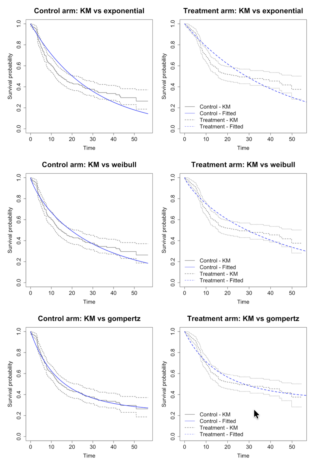
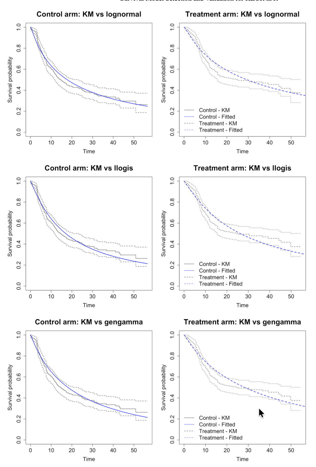
Gompertz has favorable AIC and generally acceptable graphical fit within the observed period, but log-normal and log-logistic also remain plausible on some diagnostics. Keep a set of candidate models rather than declare Gompertz uniquely best. Choose a base-case model by weighing follow-up completeness and clinical plausibility of each extrapolated tail. Use that judgment before residual-based confirmation.
Step 3.3 Q-Q plots for right-censored data
Q-Q plots help determine whether specific distribution families fit the observed data.
Below are the Q-Q plots for the control arm. You can generate similar plots for the treatment arm to assess candidate distributions across both study groups.
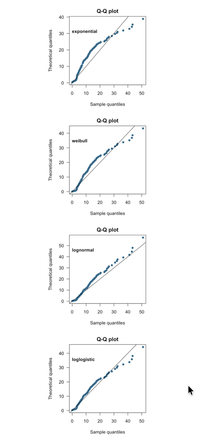
The censored Q–Q plots show departures from the reference line for each evaluated family, especially at later quantiles where information may be sparse. These plots do not clearly identify a single preferred distribution and should be treated as screening evidence alongside arm-specific hazard plots, residual diagnostics, AIC/BIC, and clinical plausibility. This implementation cannot evaluate Gompertz due to software limitations, so assess it using other diagnostics. Use these plots as one input before residual checking.
Step 3.4 Residual plots (Cox-Snell)
Residual plots can detect systematic lack of fit in candidate models.
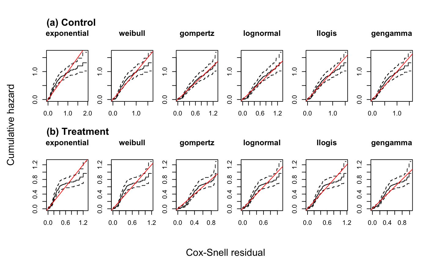
For a well-fitting model, the estimated cumulative hazard of the Cox–Snell residuals should lie approximately along the 45° line. Several candidates track the line over much of the observed range, with differing localized departures and increasing uncertainty toward the tail. These plots provide no definitive basis for selecting a particular distribution alone and should be interpreted with other diagnostics. Use them as a final internal fit check before external validity.
Step 4. Evaluate external validity & decision uncertainty
To assess how different survival models affect extrapolated survival estimates, generate long-term survival predictions for each fitted model and compare them graphically. Assume a constant treatment effect beyond the observed follow-up period. This shifts the analysis from internal fit to long-term impact.
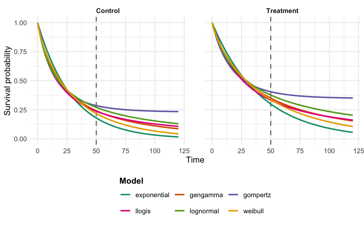
Do not consider extrapolated curves validated solely because they fit trial data. For each plausible model, report long-term survival and hazard predictions at decision-relevant time points, and compare them with relevant registries, longer-term studies, background mortality, biological expectations, and clinical-expert judgment. Discuss comparability and limitations of each external source. Use these comparisons before choosing the preferred extrapolation.
The base-case extrapolation assumes constant treatment effect throughout the period of interest, but this assumption should be critically evaluated in light of treatment-effect duration. Because post-trial relative effects are uncertain, evaluate at least three scenarios: treatment effect stops at the end of observed follow-up, wanes over a clinically justified period, or persists over the lifetime horizon. Inform assumptions with observed hazards, mechanism of action, and clinical advice. Use these scenarios to test decision uncertainty.
Step 5.Model selection & validation summary
Step 5.1 Model selection rationale
| Model | Hazard / structural evidence | KM graphical fit | Q-Q diagnostic | Cox-Snell diagnostic | AIC; ΔAIC | External plausibility | Provisional conclusion |
|---|---|---|---|---|---|---|---|
| Exponential | Constant-hazard assumption not convincingly supported | Less favorable than Gompertz, log-normal, and log-logistic | Moderate deviation, particularly during mid-to-late follow-up | Less favorable than leading models; arm-specific departures observed | 2215.113; 41.482 | Not assessed | Not preferred based on internal fit |
| Weibull | Monotonic hazard structure potentially plausible | Less favorable than Gompertz, log-normal, and log-logistic | Moderate deviation, particularly during mid-to-late follow-up | Less favorable than leading models | 2204.574; 30.943 | Not assessed | Structurally plausible, but with relatively weak internal-fit support |
| Gompertz | Monotonic hazard structure potentially plausible | Best or among the best graphical fits | Not evaluated due to GofCens limitation | Better fit in the control arm and best fit in the treatment arm | 2173.631; 0.000 | Not assessed | Provisional preferred model based on internal fit only |
| Log-normal | Not assessed in the hazard-structure analysis | Among the better graphical fits | Moderate deviation, particularly during mid-to-late follow-up | Better fit in the control arm; treatment-arm fit inferior to Gompertz | 2198.150; 24.519 | Not assessed | Potential alternative, but with weaker overall internal-fit support |
| Log-logistic | Not assessed in the hazard-structure analysis | Among the better graphical fits | Moderate deviation, particularly during mid-to-late follow-up | Better fit in the control arm; treatment-arm fit inferior to Gompertz | 2179.306; 5.675 | Not assessed | Principal alternative for structural sensitivity analysis, subject to long-term plausibility |
| Generalized gamma | Not assessed in the hazard-structure analysis | Among the better graphical fits in later KM comparisons | Not evaluated | Not evaluated | 2191.250; 17.619 | Not assessed | Evidence incomplete; further diagnostics required before assigning a scenario role |
Model selection should not rely on a single diagnostic. Synthesize structural assumptions, graphical fit, diagnostic plots, and information criteria to reach a provisional conclusion. Then confirm long-term extrapolation remains externally plausible before final selection. This summary ties earlier checks together.
Step 5.2 Structural uncertainty and scenario analysis
Use the most clinically credible model as the base case, but retain other plausible distributions and modeling structures as scenarios. Vary survival distribution, PH versus arm-specific or time-varying effects, treatment-effect duration, and, where indicated, piecewise or flexible modeling. Report the effect on extrapolated mean survival and cost-effectiveness outcomes; represent parameter uncertainty within each scenario probabilistically. This completes the uncertainty assessment after model selection.